[Understanding Riemannian Geometry] 2. From the Pythagorean Theorem to the Riemannian Metric

【理解黎曼几何】2. 从勾股定理到黎曼度量 苏剑林 · 2016-10-14 · Mathematics transform geometry riemannian geometry

The Riemannian Metric

Geometry, in English, originally meant land surveying. And if you're surveying, you need a reference frame, and you need a way to compute distances.

Once we have a reference frame, we can set up a coordinate system and write down the coordinates of every point. As for computing distances, we have the great Pythagorean theorem:

$$ds^2 = dx^2 + dy^2 \tag{1} $$

But here we've glossed over two issues.

The first issue is that we don't necessarily have to use a Cartesian coordinate system. If we use polar coordinates instead, then it should be

$$ds^2 = dr^2 + r^2 d\theta^2 \tag{2} $$

From this we can guess that the most general form should be

$$ds^2 = E(x^1, x^2)(dx^1)^2 + 2F(x^1, x^2)dx^1 dx^2 + G(x^1, x^2)(dx^2)^2 \tag{3} $$

Here $x^1,x^2$ are generalized coordinates, and we use superscripts rather than subscripts to index them, in order to stay consistent with the notation of traditional textbooks. What does this formula mean? Actually it's quite simple: just as there's no reason to demand that the whole world use RMB, there's no need to require that the same coordinate system be used everywhere in the world. A more sensible approach is to let each location use its own coordinate system (a local coordinate system), and then give the local rule for computing distances. So the formula above is precisely saying: at position $(x^1, x^2)$, the formula (the local Pythagorean theorem) for computing the length of the vector $(dx^1, dx^2)$ is $ds^2 = E(x^1, x^2)(dx^1)^2 + 2F(x_1, x_2)dx^1 dx^2 + G(x^1, x^2)(dx^2)^2$. More below.

The second issue is that, of course, we're not only interested in the 2D plane — we also want to study $n$-dimensional spaces. So the most general formula is

$$ds^2 = g_{\mu\nu}(\boldsymbol{x}) dx^{\mu} dx^{\nu} \tag{4} $$

Here $\boldsymbol{x}=(x^1,x^2,\dots,x^n)$, and we're using the Einstein summation convention, i.e., repeated upper and lower indices in a monomial imply summation. $g_{\mu\nu}$ is exactly what we call the Riemannian metric. We can choose it to be symmetric, i.e. $g_{\mu\nu}=g_{\nu\mu}$, without changing the form of $ds^2$, and the whole $ds^2$, as discussed above, is simply the different way of computing distance used at different locations in a high-dimensional space. Here, we've restored the "measurement" meaning of geometry.

On the other hand, the Riemannian metric can also be seen as a measurement standard. Just as different countries have different currencies, if there's a formula that converts any country's currency into an equivalent amount of gold, then the problem of comparing different currency amounts is solved. The Riemannian metric plays a similar role: rather than saying it gives a different way of computing distances at different locations, it's more accurate to say that it unifies the ways of computing distances across all locations.

Incidentally, it's worth noting that, purely from the standpoint of defining a distance, we don't actually have to use a quadratic form — cubic forms, quartic forms, or even more complicated forms could work too. But for the sake of practical value, we only study the quadratic case. Even so, there are already more problems than we could ever finish studying.

Some Examples

Under what circumstances do we get (or need) a non-constant Riemannian metric? As we've already seen, converting Cartesian coordinates to polar coordinates produces a non-constant Riemannian metric. In other words, even in flat space, as soon as we use a curvilinear coordinate system, a non-constant Riemannian metric appears.

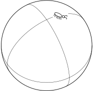Ant on a sphere

Beyond that, the Riemannian metric of a curved space is necessarily non-constant. Are there any concrete examples? The most classic one should be the two-dimensional sphere (note: the two-dimensional sphere, not three-dimensional spherical coordinates — don't get them confused). Taking the radius to be 1, the spherical coordinates are

$$\left\{\begin{aligned}&x=\sin\theta\cos\varphi\\ &y=\sin\theta\sin\varphi\\ &z=\cos\theta\end{aligned}\right. \tag{5} $$

and its Riemannian metric is then

$$ds^2=dx^2+dy^2+dz^2=d\theta^2+\sin^2\theta d\varphi^2 \tag{6} $$

Ant on an isothermal surface

Another very vivid example, which I learned from The Feynman Lectures on Physics, Volume II: suppose we're in a flat space, but the temperature varies from place to place. If we use a ruler with a very large thermal expansion coefficient as our measuring tool, what happens? In places with high temperature, the ruler expands, so the measured result becomes smaller; conversely, in places with low temperature, the ruler shrinks, so the measured result becomes larger. The same actual distance might measure as 50cm in a hot region but 100cm in a cold region, so we need a non-constant metric to unify these — either multiply the 50 by 2, or divide the 100 by 2, or multiply 50 by 4 while multiplying 100 by 2, and so on. It's not hard to guess that the Riemannian metric in this case should take the form (consider both the 2D and 3D cases):

$$ds^2 = f(x,y,z)(dx^2+dy^2+dz^2) \tag{7} $$

This gives rise to the appearance of a curved space — except that here it's not space itself that is "curved," but rather the ruler that is "curved." This example also appears in The Feynman Lectures on Gravitation; according to Feynman, it was invented by a student of Robertson's. Because of its obvious physical meaning, it's also called "isothermal parameters" or an "isothermal coordinate system." In fact, this is somewhat analogous to the idea that "motion is relative": the appearance of a curved space might be due to the space itself being curved (as with the sphere), or it might be due to the ruler being "curved" (as with the thermally expanding ruler) — but mathematically, the results are the same.

Local Cartesian Coordinate Systems

Now let's try to describe the Riemannian metric in matrix form. Write $\boldsymbol{g}=g_{\mu\nu}, \boldsymbol{x}=x^{\alpha}, d\boldsymbol{x}=dx^\alpha$, where vectors are column vectors, and we don't distinguish between a vector and its components. Then the Riemannian metric can be written as

$$ds^2 = d\boldsymbol{x}^T \boldsymbol{g}d\boldsymbol{x} \tag{8} $$

Notice that the matrix $\boldsymbol{g}$ is symmetric, so in general it can be decomposed as $\boldsymbol{h}^T \boldsymbol{h}$, where $\boldsymbol{h}$ is a matrix of the same order as $\boldsymbol{g}$. In that case

$$ds^2 = d\boldsymbol{x}^T \boldsymbol{h}^T \boldsymbol{h} d\boldsymbol{x}=\left(\boldsymbol{h}d\boldsymbol{x}\right)^T\left(\boldsymbol{h}d\boldsymbol{x}\right)=\left|\boldsymbol{h}d\boldsymbol{x}\right|^2 \tag{9} $$

In other words, this ultimately reduces to the norm of $\boldsymbol{h}d\boldsymbol{x}$, and this norm agrees with the Pythagorean theorem of flat space. We can think of the matrix $\boldsymbol{h}$ as precisely describing the local coordinate system: the vector $d\boldsymbol{x}$ in the coordinate system $\boldsymbol{h}$ is exactly equivalent to the vector $\boldsymbol{h}d\boldsymbol{x}$ in the local Cartesian coordinate system. In other words, $\boldsymbol{h}$ is the transformation matrix (the Jacobian matrix) from the local coordinate system to the local Cartesian coordinate system.

Once we have the transformation to Cartesian coordinates, we can define many geometric quantities, all of which extend naturally from flat space. For instance, given a vector $\boldsymbol{A}=A^{\mu}$, its squared norm is

$$|\boldsymbol{h}\boldsymbol{A}|^2 = \boldsymbol{A}^T \boldsymbol{h}^T\boldsymbol{h}\boldsymbol{A}=\boldsymbol{A}^T \boldsymbol{g}\boldsymbol{A}=g_{\mu\nu}A^{\mu}A^{\nu} \tag{10} $$

Given two vectors $\boldsymbol{A}$ and $\boldsymbol{B}$, their inner product is

$$\left(\boldsymbol{h}\boldsymbol{A}\right)^T \left(\boldsymbol{h}\boldsymbol{B}\right)= \boldsymbol{A}^T \boldsymbol{h}^T\boldsymbol{h}\boldsymbol{B}=\boldsymbol{A}^T \boldsymbol{g}\boldsymbol{B}=g_{\mu\nu}A^{\mu}B^{\nu} \tag{11} $$

If you like, you can also define the angle $\theta$ between them as:

$$\theta=\arccos \frac{g_{\mu\nu}A^{\mu}B^{\nu}}{\sqrt{g_{\mu\nu}A^{\mu}A^{\nu}}\sqrt{g_{\mu\nu}B^{\mu}B^{\nu}}} \tag{12} $$

Likewise, we can compute the area of the parallelogram spanned by the two vectors $\boldsymbol{A}$ and $\boldsymbol{B}$:

$$\left|\boldsymbol{h}\boldsymbol{A}\right| \times \left|\boldsymbol{h}\boldsymbol{B}\right|\times \sin\theta = \sqrt{(g_{\mu\nu}A^{\mu}A^{\nu})(g_{\mu\nu}B^{\mu}B^{\nu})-(g_{\mu\nu}A^{\mu}B^{\nu})^2} \tag{13} $$

If we want to compute a (hyper)volume integral, the volume element is

$$\det(\boldsymbol{h})\prod_{\alpha} dx^{\alpha} = \sqrt{\det(\boldsymbol{g})} \prod_{\alpha} dx^{\alpha} = \sqrt{g}d\Omega \tag{14} $$

Here $g$ is shorthand for $\det(\boldsymbol{g})$, and $d\Omega$ is shorthand for $\prod_{\alpha} dx^{\alpha}$; note that we have $\det(\boldsymbol{g})=det(\boldsymbol{h}^T \boldsymbol{h})=(\det(\boldsymbol{h}))^2$. $\sqrt{g}$ is in fact just a volume scaling factor. With this result in hand, we can write: given $n$ vectors $\boldsymbol{A}^1,\boldsymbol{A}^2,\dots,\boldsymbol{A}^n$, written as column vectors, the hypervolume of the parallel $n$-dimensional body they span is

$$\sqrt{g}\det(\boldsymbol{A}^1,\boldsymbol{A}^2,\dots,\boldsymbol{A}^n)\tag{15}$$

Here $(\boldsymbol{A}^1,\boldsymbol{A}^2,\dots,\boldsymbol{A}^n)$ means arranging these $n$ column vectors into a $n\times n$ matrix.