Perturbation methods for difference equations

差分方程的摄动法 苏剑林 · 2016-08-04 · Mathematics perturbation difference equation

I've recently been thinking hard about some natural language processing problems and some nonlinear analysis problems, and haven't had time to write up a summary, for which I apologize. This post is about a perturbation scheme for first-order nonlinear difference equations (higher-order ones can of course be handled similarly). In theory, this method can produce explicit asymptotic solutions for arbitrary first-order nonlinear difference equations.

Nonlinear difference equations

For a general first-order nonlinear difference equation

$$\begin{equation}\label{chafenfangcheng}x_{n+1}-x_n = f(x_n)\end{equation}$$

it's generally the case that difference equations rarely admit analytic solutions, so we need tools like asymptotic analysis to understand the properties of nonlinear difference equations. Very often, the first thing we try is to replace the difference with a derivative, obtaining the differential equation

$$\begin{equation}\label{weifenfangcheng}\frac{dx}{dn}=f(x)\end{equation}$$

as an approximation to the difference equation $\eqref{chafenfangcheng}$. The reason for doing this, aside from the fact that differential equations often have relatively simple explicit solutions, is that the differential equation $\eqref{weifenfangcheng}$ approximately preserves some important properties of the difference equation $\eqref{chafenfangcheng}$, such as its asymptotic behavior. For example, consider the discrete logistic growth model:

$$\begin{equation}\label{zuzhizengzhang}x_{n+1}=(1+\alpha)x_n -\beta x_n^2\end{equation}$$

The corresponding differential equation (replacing the difference with a derivative) is:

$$\begin{equation}\frac{dx}{dn}=\alpha x -\beta x^2\end{equation}$$

Solving this equation gives

$$\begin{equation}x_n = \frac{\alpha}{\beta+c e^{-\alpha n}}\end{equation}$$

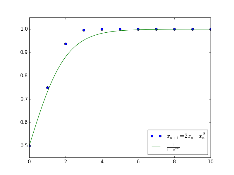
where $c$ is an arbitrary constant. This result already gives a rough picture of how the solution of the original difference equation $\eqref{zuzhizengzhang}$ behaves, and it successfully captures the eventual asymptotic limit $x_n \to \frac{\alpha}{\beta}$. The figure below compares the solution of the differential equation with the solution of the difference equation when $\alpha=\beta=1$ and $c=1$ (i.e., $x_0=\frac{1}{2}$).

Perturbation methods for difference equations 1

The question now is: given that the solution of the differential equation already serves as a well-behaved approximate solution, can we build on it and add correction terms to improve the accuracy? more

General scheme

We introduce a parameter $q$ and consider the more general difference equation

$$\begin{equation}\label{yibanchafenfangcheng}x_{n+q}-x_n = q f(x_n)\end{equation}$$

When $q=1$, this is exactly the difference equation $\eqref{chafenfangcheng}$ we're considering, while when $q\to 0$, it becomes the differential equation

$$\begin{equation}\frac{dx}{dn}=f(x)\end{equation}$$

Note that since we've introduced $q$, the specific form of $x_n$ depends on $q$; in other words, $x_n$ is actually also a function of $q$, which we write explicitly as $x_{n,q}$, i.e.

$$\begin{equation}\label{yibanchafenfangcheng2}x_{n+q,q}-x_{n,q}=qf(x_{n,q})\end{equation}$$

What we ultimately care about is $x_n\equiv x_{n,1}$. To solve this equation step by step, we imagine expanding $x_{n,q}$ as a power series in $q$:

$$\begin{equation}x_{n,q}=\sum_{k=0}^{\infty}a^{(k)}_n q^n\end{equation}$$

where

$$\begin{equation}a_n^{(k)} = \frac{1}{k!}\left.\frac{\partial^k x_{n,q}}{\partial q^k}\right|_{q=0},\quad k=0,1,2,\dots\end{equation}$$

The remaining problem is how to find each $a_n^{(k)}$.

Step-by-step expansion

Differentiating both sides of equation $\eqref{yibanchafenfangcheng2}$ with respect to $q$ (taking the total derivative with respect to $q$), we get

$$\begin{equation}\label{qiudao}\frac{\partial x_{n+q,q}}{\partial n}+\frac{\partial x_{n+q,q}}{\partial q}-\frac{\partial x_{n,q}}{\partial q}=f(x_{n,q})+q\frac{\partial f}{\partial x_{n,q}}\frac{\partial x_{n,q}}{\partial q}\end{equation}$$

I should clarify: when we write

$$\begin{equation}\frac{\partial x_{n+q,q}}{\partial q}\end{equation}$$

by default this means differentiating only with respect to the second variable $q$, not with respect to $q$ inside the first variable $n+q$. Now setting $q=0$, we get

$$\begin{equation}\label{qiudao-q-0}\frac{\partial x_{n,0}}{\partial n}=f(x_{n,0})\end{equation}$$

which is exactly the differential equation $\eqref{weifenfangcheng}$ serving as the first-order approximation.

Next, we again differentiate $\eqref{qiudao}$ with respect to $q$

$$\begin{equation}\label{qiudao2}\begin{aligned}&\frac{\partial^2 x_{n+q,q}}{\partial n^2}+2\frac{\partial^2 x_{n+q,q}}{\partial n \partial q}+\frac{\partial^2 x_{n+q,q}}{\partial q^2}-\frac{\partial^2 x_{n,q}}{\partial q^2}\\ =&2\frac{\partial f}{\partial x_{n,q}}\frac{\partial x_{n,q}}{\partial q}+q\frac{\partial^2 f}{\partial x_{n,q}^2}\left(\frac{\partial x_{n,q}}{\partial q}\right)^2+q\frac{\partial f}{\partial x_{n,q}}\frac{\partial^2 x_{n,q}}{\partial q^2}\end{aligned}\end{equation}$$

and let $q=0$, to obtain

$$\begin{equation}\label{qiudao2-q-0}\frac{\partial^2 x_{n,0}}{\partial n^2}+2\frac{\partial}{\partial n}\left(\frac{\partial x_{n,0}}{\partial q}\right)=2\frac{\partial f}{\partial x_{n,0}}\frac{\partial x_{n,0}}{\partial q}\end{equation}$$

Here the term $\frac{\partial^2 x_{n,0}}{\partial n^2}$ can be computed by substituting in the $x_{n,0}$ obtained in the previous step, so this is a first-order linear differential equation in $\frac{\partial x_{n,0}}{\partial q}$, which is also solvable. This process can be continued indefinitely, progressively improving the accuracy. The subsequent expressions get too messy to write out here, but they can be handled with Mathematica.

Discrete logistic growth model

It's easier to explain the process with a concrete example. Let's again consider the logistic growth model $\eqref{zuzhizengzhang}$. After introducing the parameter $q$, the equation becomes

$$\begin{equation}x_{n+q,q}-x_{n,q}=q\alpha x_{n,q}-q\beta x_{n,q}^2\end{equation}$$

Here $f(x)=\alpha x - \beta x^2$, and the corresponding equation $\eqref{qiudao-q-0}$ is

$$\begin{equation}\frac{\partial x_{n,0}}{\partial n}=\alpha x_{n,0}-\beta x_{n,0}^2\end{equation}$$

We've already found the solution, which is

$$\begin{equation}x_{n,0}=\frac{\alpha}{\beta+c e^{-\alpha n}}\end{equation}$$

This is the zeroth-order approximation. Correspondingly, the associated equation $\eqref{qiudao2-q-0}$ is

$$\begin{equation}\frac{\partial^2 x_{n,0}}{\partial n^2}+2\frac{\partial}{\partial n}\left(\frac{\partial x_{n,0}}{\partial q}\right)=2(\alpha-2\beta x_{n,0})\frac{\partial x_{n,0}}{\partial q}\end{equation}$$

with solution (obtained using Mathematica and then cleaned up by hand, having already set $\frac{\partial x_{0,0}}{\partial q}=0$)

$$\begin{equation}\frac{\partial x_{n,0}}{\partial q}=\left(\frac{\alpha}{\beta+ce^{-\alpha n}}\right)^2\left(\frac{1}{2}\alpha n-\ln \frac{\beta+c}{\beta+ce^{-\alpha n}}\right)ce^{-\alpha n}\end{equation}$$

Hence we have

$$\begin{equation}x_{n,q}\approx \frac{\alpha}{\beta+c e^{-\alpha n}}+q\left(\frac{\alpha}{\beta+ce^{-\alpha n}}\right)^2\left(\frac{1}{2}\alpha n-\ln \frac{\beta+c}{\beta+ce^{-\alpha n}}\right)ce^{-\alpha n}\end{equation}$$

as well as

$$\begin{equation}x_n\equiv x_{n,1}\approx \frac{\alpha}{\beta+c e^{-\alpha n}}+\left(\frac{\alpha}{\beta+ce^{-\alpha n}}\right)^2\left(\frac{1}{2}\alpha n-\ln \frac{\beta+c}{\beta+ce^{-\alpha n}}\right)ce^{-\alpha n}\end{equation}$$

This is its first-order approximation. The figure below compares this zeroth-order and first-order approximate solution against the exact value, when $\alpha=\beta=1$ and $c=1$ (i.e., $x_0=\frac{1}{2}$). As you can see, compared with the zeroth-order approximation, the first-order approximation almost coincides with the exact value.

Perturbation methods for difference equations 2

This example also illustrates a characteristic of the perturbation method: although one can, in principle, keep going, and each step is integrable, the resulting integrals can become so complicated as to be practically unusable.

A brief remark

In theory, this perturbation scheme can be used to find approximate solutions for any first-order difference equation. Whether it's actually practical in real applications, of course, needs to be judged case by case.

First, if the solution of the zeroth-order (nonlinear) differential equation is already too complicated, this method quickly becomes unworkable. Second, although each step only produces, in principle, a solvable first-order inhomogeneous linear differential equation, actually solving that differential equation is far from trivial, and often each additional step doubles both the time and effort required.

Finally, it's worth noting that the way we introduce the parameter isn't limited to the form used in $\eqref{yibanchafenfangcheng2}$ — it can also be simplified according to the specific problem at hand. For example, in the article Implicit Function Solution of a Nonlinear Difference Equation, we have

$$\begin{equation}x_{n+1}=x_n+3+\frac{3}{x_n}+\frac{1}{x_n^2},\,x_1=1\end{equation}$$

and the parameter can be introduced as

$$\begin{equation}x_{n+q,q}=x_{n,q}+3+\frac{3q}{x_{n,q}}+\frac{q^2}{x_{n,q}^2},\,x_1=1\end{equation}$$

This yields the same asymptotic solution as the one found in the article Implicit Function Solution of a Nonlinear Difference Equation. This illustrates the essence of the perturbation method: using the parameter $q$ to identify the order of each term, so that the approximation can proceed level by level. And just as with the choice of parameter, what counts as "order" is, to a large extent, a matter of convention.