A Brief Exploration of OCR Technology: 3. Feature Extraction (1)

OCR技术浅探：3. 特征提取(1) 苏剑林 · 2016-06-18 · Machine Learning image OCR feature clustering text

As the first step in an OCR system, feature extraction aims to identify the features of candidate text regions in an image, so that we can perform text localization in step two and recognition in step three. In this part, we focus on mimicking how the human eye processes images and Chinese characters, taking an innovative route in both image processing and character localization. This part of the work is the core of the entire OCR system, and also the core of our work.

Most traditional text segmentation approaches follow the pipeline of "edge detection + erosion/dilation + connected component detection," as in paper [1]. However, when performing edge detection on images with complex backgrounds, the background produces too many edges (i.e., increased noise), while the edge information of the text is easily overlooked, leading to degraded performance. If erosion or dilation is then applied, the background region and the text region tend to fuse together, making things even worse. (In fact, we went quite far down this road—we even wrote our own edge detection functions to handle this. After extensive testing, we ultimately decided to abandon this approach.)

Therefore, in this article, we abandon edge detection and erosion/dilation altogether, and instead obtain fairly good text-region features through clustering, segmentation, denoising, pooling, and other steps. The overall pipeline is roughly as shown in Figure 2. These features can even be fed directly into the text recognition model without any additional processing. Since every step of our pipeline is backed by a corresponding theoretical foundation, the reliability of the model is well assured.

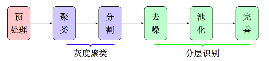Figure 2: Overview of the feature extraction pipeline

For this part of the experiments, we use Figure 3 to demonstrate our results. This image is characterized by medium size, a flashy background, rich colors, and a layout in which text is mixed with images in an irregular format—a fairly typical e-commerce promotional image. As can be seen, the key challenge in processing this image is distinguishing the image region from the text region, i.e., identifying and removing the rice cooker on the right, and keeping only the text region.

Figure 3: Xiaomi rice cooker promotional image

Image preprocessing

First, we read the original image in as a grayscale image, obtaining a grayscale matrix $M$ of size $m\times n$, where $m,n$ is the height and width of the image. Reading the image this way results in lower dimensionality than reading in a color RGB image directly, while not causing any noticeable loss of textual information. Converting to grayscale essentially merges the three channels of the original RGB image into a single channel using the following formula:

$$Y = 0.299R+0.587 G+0.114 B\tag{1}$$

The grayscale version of Figure 3 is shown below.

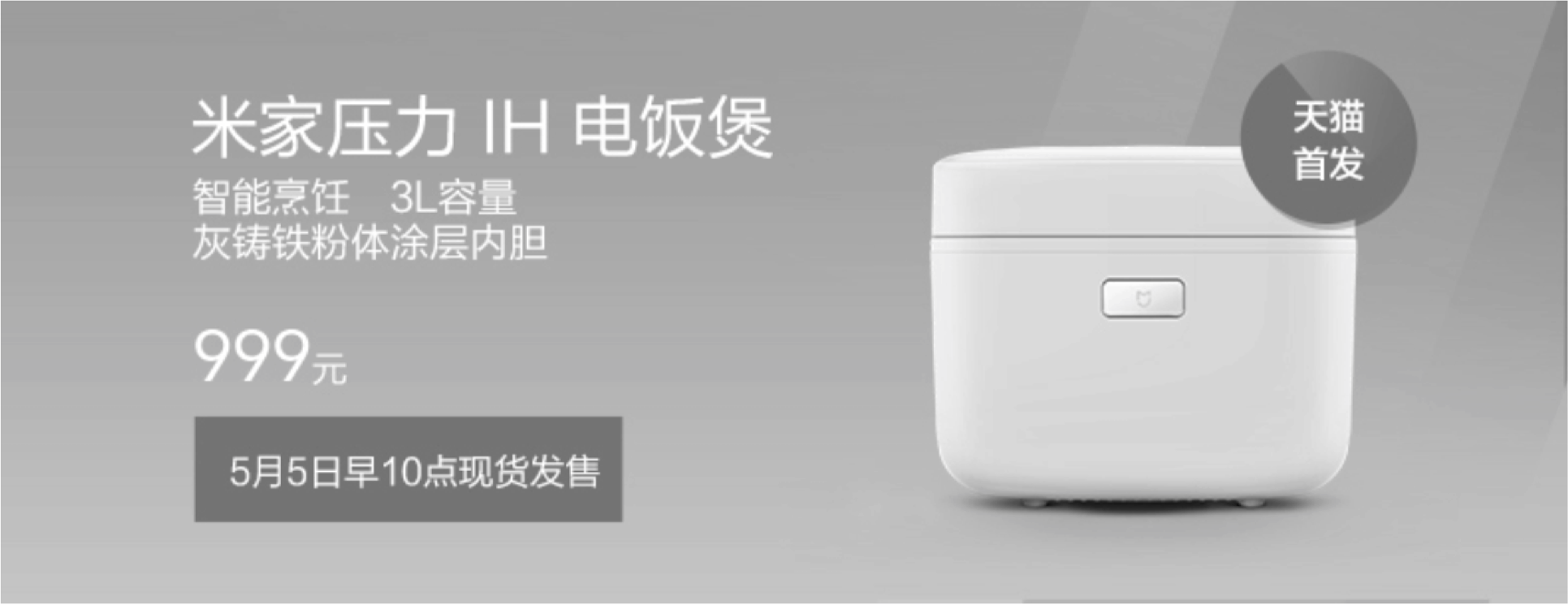Grayscale image

The image itself is not very large, so processing it directly would make the strokes of the text too thin, causing them to be mistaken for noise. Therefore, to ensure that the text strokes have sufficient thickness, we first enlarge the image. In our experiments, enlarging the image to twice its original size generally gives good results.

However, after enlarging the image, the contrast between text and background is reduced. This is because image enlargement uses an interpolation algorithm to fill in the missing pixels in the gaps. At this point, we need to increase the contrast accordingly. Through testing, we found that in most images, using a "power-law transformation" with an exponent of 2 works well. The power-law transformation is given by

$$x \mapsto x^r\tag{2}$$

where $x$ represents an element of the matrix $M$, and $r$ is the exponent, which we choose to be 2 here. The result then needs to be mapped to the $[0,255]$ interval:

$$x \mapsto \frac{x-M_{min}}{M_{max}-M_{min}}\times 255\tag{3}$$

where $M_{max},M_{min}$ are the maximum and minimum values of the matrix $M$. After this processing, the image looks like the figure below.

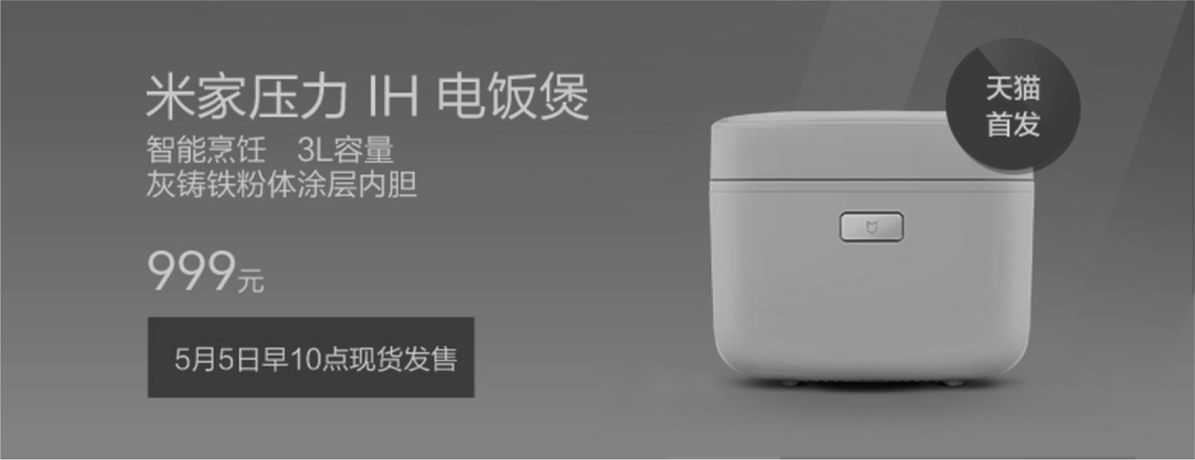Power-law transformation

Grayscale clustering

Next, we cluster the colors in the image. This clustering step is based on two empirical facts:

1.
Grayscale resolution
The grayscale resolution of the human eye is roughly 40, so pixel values of 254 and 255, for example, both appear to us simply as white;
2.
Design principles
According to common aesthetic principles—as followed, for instance, in poster design or clothing coordination—the number of colors used in a coordinated color scheme (clothing, posters, etc.) is generally no more than three.

Put more plainly, although the grayscale range spans $[0,255]$ levels, the overall tones we can actually perceive are usually few. Therefore, we can group nearby gray levels into a single class, thereby reducing the color distribution and effectively lowering noise.

In fact, clustering is a process of adaptive multi-level thresholding based on the characteristics of the image, avoiding the information loss caused by traditional simple binarization. Since we need to automatically determine the number of clusters, traditional clustering methods such as KMeans were ruled out for us. Moreover, through testing, we found that other feasible clustering methods, such as MeanShift, suffer from drawbacks such as slow speed. We therefore designed our own clustering method based on the idea of "kernel density estimation," clustering by finding the extrema of the color density.

Kernel density estimation

For the preprocessed image, we can count the number of occurrences of each gray level, obtaining the frequency distribution histogram shown in Figure 5:

Figure 5: Gray-level statistics of the preprocessed image

As can be seen, the distribution of gray levels forms several prominent peaks, in other words, there is a certain tendency toward clustering. However, the results of the histogram statistics are discrete, and a smooth result is easier for us to analyze and is also more convincing. The method for smoothing the statistical result is kernel density estimation.

Kernel density estimation is a non-parametric estimation method proposed by Rosenblatt and Parzen, and it has received a great deal of attention in both statistical theory and applications [2]. Of course, it can also simply be regarded as a way of smoothing a function. When we estimate the probability (density) of a certain value occurring based on a large amount of data, what we are effectively computing is:

$$\hat{p}(x)=\frac{1}{nh}\sum_{i=1}^n K\left(\frac{x-x_i}{h}\right)\tag{4}$$

where $K(x)$ is called the kernel function. When $h$ is taken to be 1, and $K(x)$ is taken to be

$$K\left(x\right)=\left\{\begin{aligned}&1,\,x=0\\ &0,\,x \neq 0\end{aligned}\right.\tag{5}$$

this reduces to the histogram estimate described above. The term $K(x)$ has a simple meaning: it tells us that all $x_i$ within the range $h$ are counted into $x$; exactly how they are counted is determined by $K\left(\frac{x-x_i}{h}\right)$. Clearly, the choice of $h$ has a large impact on the result; $h$ is called the bandwidth, and it primarily affects the smoothness of the result.

If $K(x)$ is discrete, the resulting estimate will also be discrete, but if $K(x)$ is smooth, the resulting estimate will likewise be relatively smooth. A commonly used smooth kernel function is the Gaussian kernel:

$$K(x)=\frac{1}{\sqrt{2\pi}}e^{-x^2/2}\tag{6}$$

The resulting estimate is also called Gaussian kernel density estimation. Here, we use Scott's rule to adaptively select $h$, but we still need to manually specify a smoothing factor, which in this article we set to 0.2. For the example image, we obtain the result shown by the red curve in Figure 6.

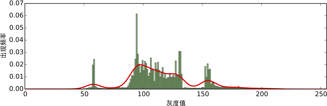Figure 6: Gaussian kernel density estimation of the frequency distribution

Maxima–minima segmentation

From Figure 6, we can further observe that the image does indeed exhibit a tendency toward clustering. This is reflected in the presence of several distinct local maxima and minima, where the maxima are located at $x=10, 57, 97, 123, 154$ and the minima at $25, 71, 121, 142$.

Therefore, a very natural clustering approach is: cluster into as many classes as there are local maxima, using the local minima as the boundaries between classes. That is, for Figure 3, the image can be divided into 5 layers, which are processed one by one. After layering, the shape of each layer is as shown in the figures below, where white represents 1 and black represents 0.

Layer 1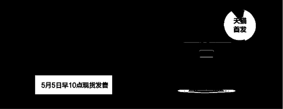Layer 2

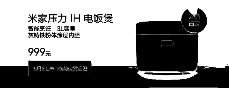Layer 3Layer 4

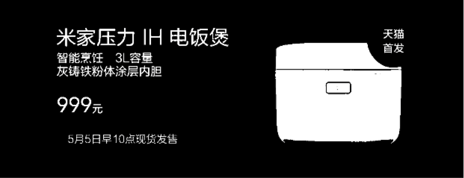Layer 5

Splitting the image into 5 layers via clustering

As can be seen, thanks to the "contrast" and "smooth gradation" assumptions, clustering via kernel density estimation can indeed successfully separate out the text layer. Moreover, this layered clustering approach requires no assumptions whatsoever about the color of the text—even when the text color matches the background color, it can still be detected effectively.