"Entropy" Cannot Be Left Alone: From Entropy, the Maximum Entropy Principle, to the Maximum Entropy Model (Part 2)

“熵”不起：从熵、最大熵原理到最大熵模型（二） 苏剑林 · 2015-12-11 · Mathematics probability extremum maximum entropy entropy

Recap of the Previous Post

In the first post, I introduced the concept of "entropy" and some of its background. The formula for entropy is

$$S=-\sum_x p(x)\log p(x)\tag{1}$$

or

$$S=-\int p(x)\log p(x) dx\tag{2}$$

And in the first post, we learned that entropy represents both uncertainty and information content — in fact, these are the same concept.

Having discussed the concept of entropy, we now turn to the "maximum entropy principle." The maximum entropy principle tells us that when we want to determine the probability distribution of a random event, if we don't have enough information to fully pin down that distribution (perhaps we don't know its type at all, or perhaps we know the type of distribution but some of its parameters remain undetermined), then the "safest" choice is the distribution that maximizes entropy.

The Maximum Entropy Principle

Admitting Our Ignorance

Many articles, when introducing the maximum entropy principle, cite the famous saying "don't put all your eggs in one basket" as a folksy way to explain the principle. However, I would humbly submit that this saying misses the point and doesn't really capture the essence of the maximum entropy principle. In my view, a more fitting explanation of the maximum entropy principle is: admit our ignorance!

How should we understand the connection between this statement and the maximum entropy principle? We already know that entropy is a measure of uncertainty; maximum entropy means maximum uncertainty. So it's clear that choosing the distribution with maximum entropy means choosing the distribution about which we are most ignorant. In other words, we admit our ignorance about the problem rather than deceiving ourselves — we may deceive each other, but we can never deceive nature.

For example, when flipping a coin, we generally assume the probabilities of heads and tails are equal. In this case, entropy is maximized, and we are in a state of maximum ignorance about the coin. But suppose someone is confident that the probability of heads is 60% and tails is 40% — that person must know that the coin has been tampered with in some way that makes heads more likely. Therefore, that person's understanding of the coin must be greater than ours, and if we lack that information, we should honestly admit our ignorance and simply assume the two probabilities are equal, rather than making subjective guesses. (After all, there are too many things we could subjectively guess — if we wrongly assume tails is more likely, we stand to lose even more.)

So, choosing the model with maximum entropy means being honest with nature, and we believe that if we are honest with nature, nature will not shortchange us in return. This is the philosophical significance of the maximum entropy principle. In addition, admitting our ignorance also means we assume we can extract the maximum amount of information from what we know, which, in a certain sense, also aligns with the principle of economy.

Estimating Probabilities

Having said all this, we still haven't actually calculated anything, and clearly words alone are not very persuasive. Let's start with the simplest problem: using the maximum entropy principle to explain why we believe the probabilities of heads and tails when flipping a coin are both $\frac{1}{2}$. Suppose the probability of heads is $p$; then the entropy is

$$S(p) = -p \log p - (1-p)\log (1-p)\tag{15}$$

Taking the derivative, we find that $S(p)$ is maximized when $p=\frac{1}{2}$, so we conjecture that the probability of each side is $\frac{1}{2}$. Similarly, one can show that according to the maximum entropy principle, when rolling a die, the probability of each face should be $\frac{1}{6}$ — this is a multivariable calculus problem. If there are $n$ possible outcomes, the probability of each outcome should be $\frac{1}{n}$.

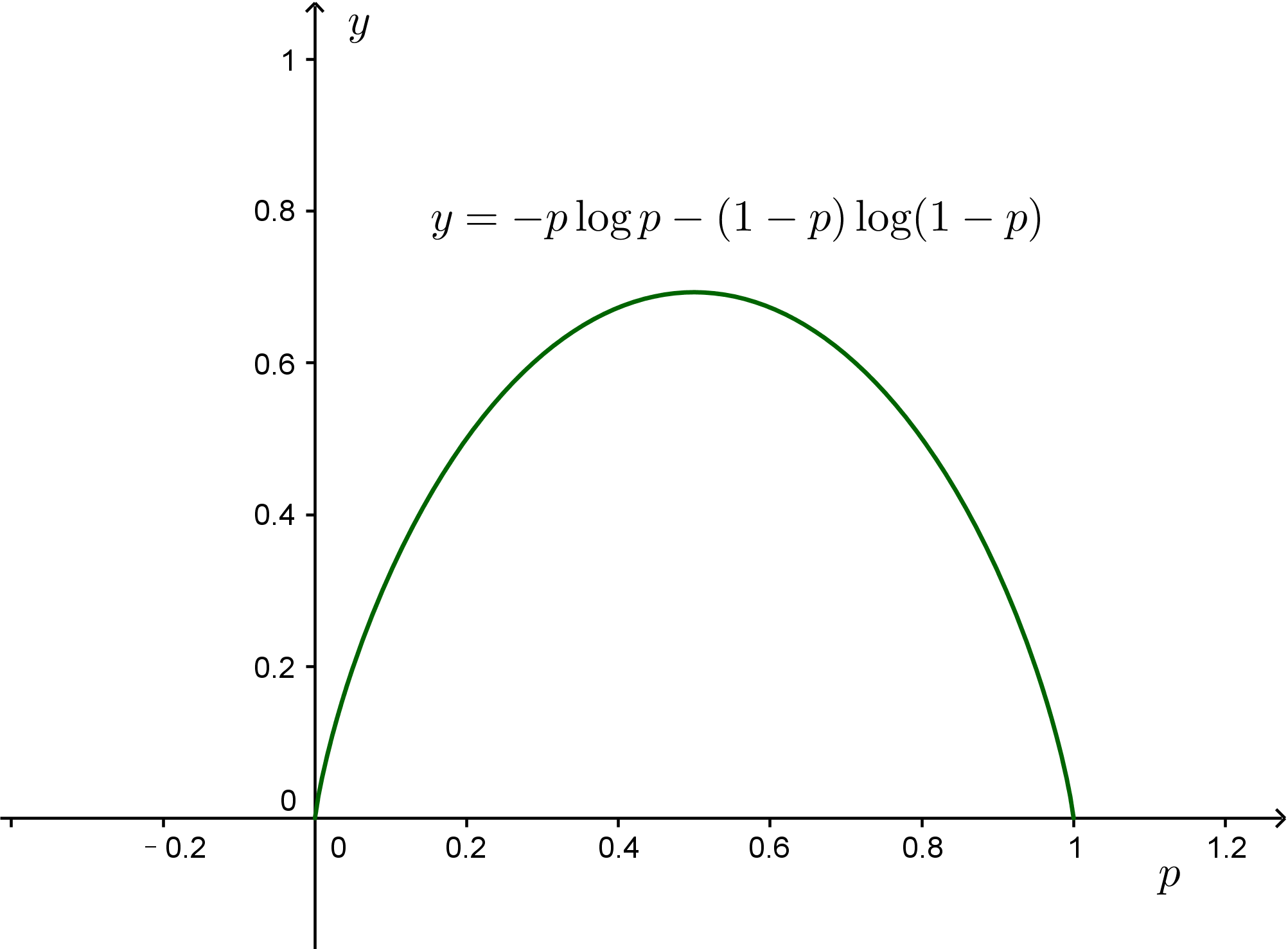Maximum entropy principle

It's worth noting that all of the above are estimates made under the assumption that we are completely ignorant. In fact, much of the time we are not that ignorant — we can use large amounts of statistics to obtain some information that refines our understanding. Consider the following example:

A fast-food restaurant offers 3 kinds of food: hamburger (1), chicken (2), and fish (3), priced at 1 yuan, 2 yuan, and 3 yuan respectively. It is known that people's average spending at this restaurant is 1.75 yuan. Find the probability that a customer buys each of these 3 foods.

Here, "people's average spending at this restaurant is 1.75 yuan" is a result obtained from extensive statistics. If we assumed we were completely ignorant, we would conclude that the probability of buying each food is $\frac{1}{3}$, but then the average spending would be 2 yuan, which doesn't match the fact that "people's average spending at this restaurant is 1.75 yuan." In other words, we are not completely ignorant about purchasing patterns at this restaurant — at the very least, we know that "people's average spending at this restaurant is 1.75 yuan," and this fact helps us estimate the probabilities more accurately.

Estimation Framework

Discrete Probability

These "facts" that help us estimate probabilities more accurately might come from our life experience, or from some kind of prior information, but regardless, they must be results obtained through statistics. Mathematically, they are described as constraints given in the form of expectations:

$$E[f(x)]=\sum_{x} p(x)f(x) = \tau\tag{16}$$

Note that although we are no longer completely ignorant, we must still admit that we are ignorant — but this is ignorance given the premise of already knowing certain facts. In mathematical terms, the problem now becomes: under $k$ constraints of the form $(16)$, find the maximum of $(1)$. For the fast-food restaurant example, $f(x)=x$, i.e.

$$\sum_{x=1,2,3}p(x)x=1.75\tag{17}$$

we seek the maximum of $-\sum_x p(x)\log p(x)$. This kind of problem is precisely a constrained extremum problem from calculus, and the method is the Lagrange multiplier method: we introduce parameters $\lambda$, so that the original problem becomes equivalent to finding the extremum of the following expression

$$-\sum_x p(x)\log p(x)-\lambda_0\left(\sum_x p(x) -1\right)-\lambda_1\left(\sum_x p(x)x -1.75\right)\tag{18}$$

In equation $(18)$, we've introduced two constraints: the first is the universal one, that all the $p(x)$ sum to 1; the second is the "fact" we've come to know. Taking derivatives, we find the extremum point at $p(1) = 0.466,p(2) = 0.318,p(3)=0.216$, at which point the entropy is maximized.

More generally, suppose there are $k$ constraints; then we need to find the extremum of the following:

$$\begin{aligned}-\sum_x p(x)\log p(x)&-\lambda_0\left(\sum_x p(x) -1\right)-\lambda_1\left(\sum_x p(x)f_1(x) -\tau_1\right)\\ &-\dots-\lambda_k\left(\sum_x p(x)f_k(x) -\tau_k\right)\end{aligned}\tag{19}$$

Equation $(19)$ can readily be solved to give

$$p(x)=\frac{1}{Z}\exp\left(-\sum_{i=1}^k \lambda_i f_i (x)\right)\tag{20}$$

Here $Z$ is the normalization factor, i.e.

$$Z=\sum_x \exp\left(-\sum_{i=1}^k \lambda_i f_i (x)\right)\tag{21}$$

Substituting equation $(20)$ into

$$\sum_x p(x)f_i(x) -\tau_i=0,\quad (i=1,2,\dots,k)\tag{22}$$

we can solve for each of the unknown $\lambda_i$ (unfortunately, for general $f_i(x)$, the above equation has no simple closed-form solution, and even numerical solutions aren't easy to obtain, which makes maximum-entropy-related models rather difficult to use in practice).

Continuous Probability

Note that equation $(19),(20),(21),(22)$ is a result derived for discrete probability; the result for continuous probability is analogous — for instance, equation $(19)$ corresponds to

$$\begin{aligned}-\int p(x)\log p(x)dx &-\lambda_0\left(\int p(x)dx -1\right)-\lambda_1\left(\int p(x)f_1(x)dx -\tau_1\right)\\ &-\dots-\lambda_k\left(\int p(x)f_k(x)dx -\tau_k\right)\end{aligned}\tag{23}$$

Finding the maximum of equation $(23)$ is in fact a problem in the calculus of variations, but since no derivative terms appear, this variational problem is essentially no different from ordinary differentiation, and the result remains

$$p(x)=\frac{1}{Z}\exp\left(-\sum_{i=1}^k \lambda_i f_i (x)\right)\tag{24}$$

and

$$Z=\int \exp\left(-\sum_{i=1}^k \lambda_i f_i (x)\right)dx\tag{25}$$

Likewise, we need to substitute equation $(24)$ into

$$\int p(x)f_i(x)dx -\tau_i=0,\quad (i=1,2,\dots,k)\tag{26}$$

to solve for each parameter $\lambda_i$.

A Continuous Example

Solving the continuous case is sometimes easier. For instance, if there's only one constraint, $f(x)=x$, i.e. we know the mean of the variable, then the probability distribution is an exponential distribution

$$p(x)=\frac{1}{Z}\exp\left(-\lambda x\right)\tag{27}$$

with normalization factor

$$\int_0^{\infty} \exp\left(-\lambda x\right) dx = \frac{1}{\lambda}\tag{28}$$

so the probability distribution is

$$p(x)=\lambda \exp\left(-\lambda x\right)\tag{29}$$

We also have a constraint

$$\tau=\int_0^{\infty} \lambda \exp\left(-\lambda x\right) x dx =\frac{1}{\lambda}\tag{30}$$

so the result is

$$p(x)=\frac{1}{\tau} \exp\left(-\frac{x}{\tau}\right)\tag{31}$$

Furthermore, if there are two constraints, namely $f_1 (x)=x,f_2(x)=x^2$, which is equivalent to knowing the mean and variance of the variable, then the probability distribution is a normal distribution (note that the normal distribution has appeared again)

$$p(x)=\frac{1}{Z}\exp\left(-\lambda_1 x-\lambda_2 x^2\right)\tag{32}$$

with normalization factor

$$\int_{-\infty}^{\infty} \exp\left(-\lambda_1 x-\lambda_2 x^2\right) dx = \sqrt{\frac{\pi}{\lambda_2}}\exp\left(\frac{\lambda_1^2}{4\lambda_2}\right)\tag{33}$$

so the probability distribution is

$$p(x)=\sqrt{\frac{\lambda_2}{\pi}}\exp\left(-\frac{\lambda_1^2}{4\lambda_2}\right) \exp\left(-\lambda_1 x-\lambda_2 x^2\right)\tag{34}$$

The two constraints are

$$\begin{aligned}&\tau_1=\int_{-\infty}^{\infty} \sqrt{\frac{\lambda_2}{\pi}}\exp\left(-\frac{\lambda_1^2}{4\lambda_2}\right) \exp\left(-\lambda_1 x-\lambda_2 x^2\right) x dx =-\frac{\lambda_1}{2\lambda_2}\\ &\tau_2=\int_{-\infty}^{\infty} \sqrt{\frac{\lambda_2}{\pi}}\exp\left(-\frac{\lambda_1^2}{4\lambda_2}\right) \exp\left(-\lambda_1 x-\lambda_2 x^2\right) x^2 dx =\frac{\lambda_1^2+2 \lambda_2}{4 \lambda_2^2} \end{aligned}\tag{35}$$

Substituting the solved result into equation $(34)$ gives

$$p(x)=\sqrt{\frac{1}{2\pi(\tau_2-\tau_1^2)}}\exp\left(-\frac{(x-\tau_1)^2}{2(\tau_2-\tau_1^2)}\right)\tag{36}$$

Note that $\tau_2-\tau_1^2$ is exactly the variance, so the result is exactly a normal distribution with mean $\tau_1$ and variance $\tau_2-\tau_1^2$!! This gives us yet another origin story for the normal distribution!