A Diagrammatic Technique for the Series Expansion of exp(1/2 t² + xt)

exp(1/2 t^2+xt)级数展开的图解技术 苏剑林 · 2015-08-13 · Mathematics series diagram

This post examines the Taylor expansion, at $t=0$, of the function of $t$

$$\exp\left(\frac{1}{2}t^2+xt\right)$$

Clearly this is not a hard problem — it can be done by hand or with software, and the answer is

$$1+x t+\frac{1}{2} \left(x^2+1\right) t^2+\frac{1}{6}\left(x^3+3 x\right) t^3 +\frac{1}{24} \left(x^4+6 x^2+3\right) t^4 + \dots$$

However, in this post I'll present a diagrammatic method of my own construction for this series, which lets us compute the leading terms of the expansion fairly intuitively and conveniently by hand. Afterward, we'll discuss where this diagrammatic technique originated and some further applications.

The diagrammatic method for the series: explanation

First, it's clear that to write out this series, the key step is to write out each term of the expansion, i.e., we need

$$f_k (x) = \left.\frac{d^k}{dt^k}\exp\left(\frac{1}{2}t^2+xt\right)\right|_{t=0}$$

$f_k (x)$ is an integer-coefficient polynomial of degree $k$ in $x$, and $k$ is the order of the expansion — also the order of differentiation.

Here, we let a "dot" represent one $x$, and "a straight line between two dots" represent "multiplication." Then $x^2$ can be represented as

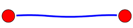x² term more

We let the number of "dots" represent the power of $f_k (x)$, so every term of $f_k (x)$ should have $k$ dots. But $f_k (x)$ isn't always of degree $k$ — in that case, we use "two dots joined by a wavy line" to represent "1." Borrowing terminology from physics, we can say these two dots have "coupled" into a constant. So the diagram below represents $x$ within $f_3(x)$:

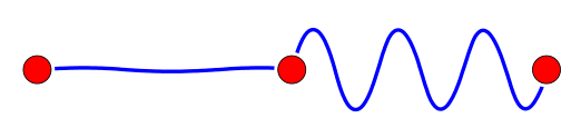x term in f3(x)

Note that the form of a term doesn't depend on the order in which the diagram is drawn — that is, the diagram below also represents $x$ within $f_3(x)$:

another representation of the x term in f3(x)

To represent the coefficient in front of a term, we append the corresponding number afterward, so the diagram below represents the term $3x$ within $f_3(x)$:

the 3x term in f3(x)

We also need one more restriction: "two wavy lines cannot appear adjacent to each other." That is, the diagram below is forbidden:

a forbidden term

Now we can readily read off the diagram below:

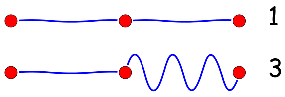f3(x)

It represents $x^3+3x$, the third-order term of the Taylor expansion. Similarly, the diagram

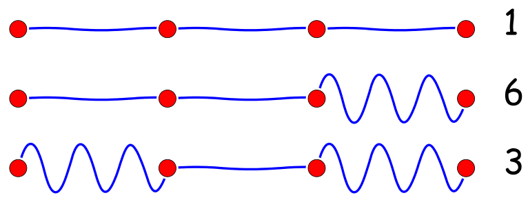f4(x)

represents $x^4+6x^2+3$, the fourth-order term of the Taylor expansion.

The diagrammatic method for the series: recursion

If this diagrammatic representation were all there was to it, it would be nothing more than an alternative way of writing the series, and wouldn't actually help us at all. However, with the help of the diagrams we can quite intuitively carry out the recursion — that is, the process of going from the order-$k$ diagram to the order-$k+1$ diagram.

Take the step from order $3$ to order $4$ as an example. The order-3 diagram is

f3(x)

The order-$4$ diagram has 4 dots, i.e., we add 1 dot. Imagine that this newly added dot emits two kinds of "signal": a straight-line signal and a wavy-line signal. Both signals probe every dot in the existing diagram, but they behave differently.

The straight-line signal

The straight-line signal is the "quit while you're ahead" type: it makes no distinction between dots, and as soon as it detects a dot, it connects to it and stops probing any further. So, after being probed by the straight-line signal, the order-3 diagram becomes

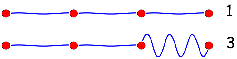probing by the straight-line signal

The wavy-line signal

The wavy-line signal, unlike the straight-line signal, is discriminating: it carefully probes every dot into which it could possibly be embedded, and embeds itself into each one in turn. So, after being probed by the wavy-line signal, the order-3 diagram becomes (the first three diagrams here are equivalent)

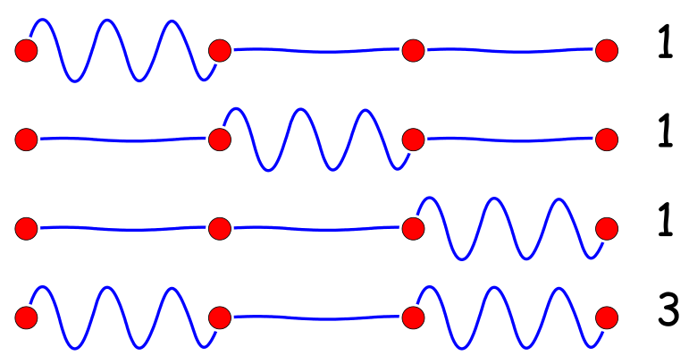probing by the wavy-line signal

Combining the results of both signals' probing, we obtain the order-4 diagram

f4(x)

which represents $x^4+6x^2+3$, the fourth-order term of the Taylor expansion.

This is just one illustration; readers are welcome to further simplify the process according to their own understanding.

The diagrammatic method for the series: application

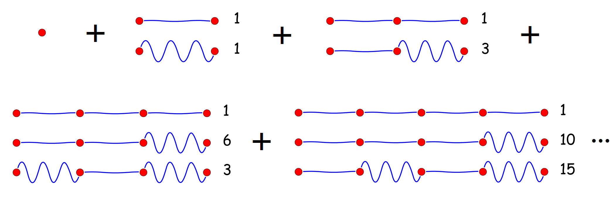
Using the recursion process described above, we can fairly quickly draw the diagram for this series

the series

The first term represents $f_1 (x) = x$, corresponding to the $xt$ term of the Taylor expansion; the second term represents $f_2 (x) = x^2 + 1$, corresponding to the $\frac{1}{2!}(x^2 + 1)t^2$ term of the Taylor expansion; the third term represents $f_3 (x) = x^3 + 3x$, corresponding to the $\frac{1}{3!}(x^3 + 3x)t^3$ term of the Taylor expansion; and so on. Hence

$$\exp\left(\frac{1}{2}t^2+xt\right)=1+x t+\frac{1}{2} \left(x^2+1\right) t^2+\frac{1}{6}\left(x^3+3 x\right) t^3 + \dots$$

Obviously, if the only goal were to expand this particular series, all this machinery would be overkill. But if we reinterpret the dots and wavy lines to mean other things, this technique could potentially prove useful in expanding much more complicated expressions. In fact, I originally worked out this method while studying the "external-source technique" (functional derivatives) used in quantum-mechanical perturbation theory. There, one needs

$$\frac{\delta^n}{\delta x^n}\exp\left[\int \left(xf+\frac{1}{2}fL^{-1}f\right)dt\right]$$

Computing functional derivatives is far more complicated than computing ordinary derivatives, so having a diagrammatic scheme like this to assist the calculation can reduce the computational burden and make it easier to derive each term. And indeed, in the context of functional derivatives, an analogous technique does exist — it amounts to coloring the dots differently to distinguish the various terms from one another. As you can imagine, there would be many more terms, and much more complicated ones, in that case. But that's a story for a future post.