A Year-Late Model: Revisiting Shredded Paper Restoration

迟到一年的建模：再探碎纸复原 苏剑林 · 2014-12-18 · Life-Feeling code Python modeling image

A Year-Late Piece of Modeling: Revisiting Shredded Paper Reconstruction

Preface: A year ago, during the national mathematical modeling competition, I tackled Problem B in a fairly rudimentary way, and afterward wrote up Shredded Paper Reconstruction: One Person's Mathematical Modeling. At the time I was simply fascinated by the problem, and after a day of work I had more or less finished the code for attachments 1 and 2, with only a vague notion of how to handle attachment 3. This year, in our mathematical modeling course, the instructor assigned this very problem as a term project, so I picked up the enthusiasm I'd had a year earlier and continued that unfinished one-person modeling exercise...

Unlike last year, this time I implemented all the code in Python — simpler, cleaner, and possibly even more efficient. Below is the full write-up.

Research Background

On October 29, 2011, the U.S. Defense Advanced Research Projects Agency (DARPA) announced the Shredder Challenge, aiming to find efficient and effective algorithms for reconstructing paper that had been shredded. [1] The competition attracted 9,000 teams from across the United States, and after more than a month, one team succeeded in fully solving the official problem.

In recent years, shredded paper reconstruction has drawn increasing attention. It demonstrates the possibility of "restoring the truth" from fragments — that is, of "decrypting" original information from broken pieces. It is also related, in a way, to "panorama stitching" in image processing, a technique that synthesizes a complete panoramic image from a number of photos taken from different angles. For these reasons, studying shredded paper reconstruction is a topic of considerable importance. more

Taking Problem B of the 2013 China Undergraduate Mathematical Contest in Modeling as our starting point, this paper presents a preliminary study of the reconstruction of some idealized shredded paper fragments, and essentially completes the reconstruction of the fragments provided officially. Our results show that reconstructing idealized shredded fragments is entirely feasible, and can be accomplished in a reasonably short amount of time.

Idealized Assumptions

We assume the shredded fragments satisfy the following idealized conditions:

1. Every fragment is a rectangle of the same size;
2. The cuts are parallel, with no tilt;
3. All fragments are face-up;
4. No fragments are missing or mixed in from elsewhere — i.e., all fragments can be assembled into one complete original image.

Model Construction

Under the idealized assumptions above, we built a mathematical model for shredded paper reconstruction. In doing so, we made use of and improved upon a greedy algorithm, and analyzed both the matching metric and the role of manual intervention.

An idealized image fragment is a rectangle, which, once pixelated, becomes a pixel matrix. To determine whether two fragments are adjacent, we mainly compare whether their edges align — that is, we compare the similarity of the edge column vectors of the pixel matrices. Regarding the choice of matching metric, we compared two different measures — distance and correlation coefficient — and ultimately settled on distance as our metric. Finally, for the assembly of attachments 3 and 4, we introduced two modes of manual intervention; the results show that both modes work well, though there remains room for further optimization.

It's worth noting that, to preserve the general applicability of the algorithm, we did not binarize the images. Although binarizing the fragment images would yield more effective processing for this particular problem, binarization is not suitable for reconstructing most other types of images (here "type" refers to the content of the fragments, which must still satisfy the idealized assumptions). Therefore, to keep our algorithm broadly applicable, we work directly with the original images rather than binarizing them first.

Greedy Algorithm

For matching fragments, we mainly used a greedy algorithm. The basic procedure is: manually select a starting fragment, compare the rightmost edge column vector of that fragment's pixel matrix against the leftmost edge column vectors of all other fragments, and choose the fragment with the highest match score. Then, starting from the newly matched fragment, repeat the process of finding the best match among the remaining fragments, and so on.

The greedy algorithm seeks local optima in the hope of reaching a global optimum; it is easy to implement and efficient. However, since it only searches for a local optimum at each step, there is no guarantee that the final result is globally optimal. In shredded paper reconstruction, this algorithm can lead to two types of anomalies:

1. Different starting points yield different assembly results.
2. When edge information is scarce, mismatches occur frequently.

To (partially) avoid these shortcomings of the greedy algorithm, we improved it by incorporating manual intervention. Testing showed that attachments 1 and 2 required no additional manual intervention, so our manual-intervention design targets only attachments 3 and 4. The details of this improvement are described in $\ref{sec:rengongganyu}$.

Matching Metric

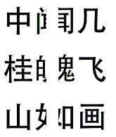Adjacent shredded fragments

As shown in the figure above, from the standpoint of image connectivity, the edge pixels of two adjacent fragments should generally be similar, or even identical. This naturally suggests using the distance between the two edge vectors as the matching metric:

$$\begin{equation}d^2=|\boldsymbol{x}-\boldsymbol{y}|^2=\sum_{i=1}^{n}(x_i-y_i)^2\end{equation}$$

If the distance between two edge vectors is 0, we can be fairly confident the two fragments match. But when the distance is large, how confident can we be that the fragments do not match? We know that ordinary images not only exhibit connectivity but also gradual variation. For a typical image, adjacent column vectors can be regarded as varying roughly linearly, which suggests that "linear correlation" might be a more appropriate way to measure the match. The formula for the linear correlation coefficient [3] is:

$$\begin{equation}\rho_{X,Y}={\mathrm{cov}(X,Y) \over \sigma_X \sigma_Y} ={E[(X-\mu_X)(Y-\mu_Y)] \over \sigma_X\sigma_Y}\end{equation}$$

The formula for the linear correlation coefficient is considerably more complex than the distance formula. We tested both metrics on the same set of fragments across various image contents, and found that, overall, the linear correlation coefficient performed better than the distance formula. However, its advantage was most apparent for photographic-content fragments (which our team generated ourselves to test the algorithm), whereas for the text-content fragments provided officially, the two metrics performed about equally well. In the end, for the sake of simplicity, we chose vector distance as our matching metric.

Manual Intervention

This section concerns attachments 3 and 4. To facilitate manual intervention, when assembling the fragments we labeled each fragment with its filename in the display, without modifying the original fragment files themselves.

First, if we directly apply the code for attachments 1 and 2 to attachment 3, we get the following result (partial view):

Initial assembly of attachment 3

All fragments end up strung together into one long strip, which contains some correctly assembled sections interspersed with quite a few mistakes. Viewed differently, the fragments have effectively been grouped into roughly 20-30 somewhat larger blocks. This means we can fix the correctly assembled portions and then reassemble these blocks instead. This reduces the workload from over 200 fragments down to just over 20 blocks. Here, a human needs to visually identify which sections have already been correctly assembled and record them in the code — effectively, this amounts to manual clustering. (We did not use an automatic clustering algorithm here; the reasons will be explained later in the difficulty analysis.)

In addition, we introduced "manual exclusion." When two fragments have very similar distances, the greedy algorithm may make a mistaken match. But such cases are not frequent — once there is enough edge information, or once fragments have already been clustered, mismatches become a low-probability event. So whenever we observe a mismatch, we can manually exclude that particular matching option, forcing the program to choose the best match among the remaining possibilities. We have good reason to believe that after a finite (and small) number of such exclusions, the program will automatically converge on the correct matches.

As further correct assembly information becomes available, it can be added to the code, followed by further exclusion and manual assembly. Repeating this process allows the reconstruction to be completed within an "acceptable" amount of time.

Problem Solutions

Here we summarize the results we obtained.

Attachments 1 and 2

We illustrate using attachment 1 as an example; the assembly code for attachment 1 is given in the appendix. First, an arbitrary starting image is specified — the $m$ value in the code — and the correct starting image (008.bmp) is then determined from the resulting assembly. The $m$ value is updated accordingly, and the assembly is rerun. Testing shows that no additional manual intervention is required. The final assembly order for attachment 1 is:

[8, 14, 12, 15, 3, 10, 2, 16, 1, 4, 5, 9, 13, 18, 11, 7, 17, 0, 6]

The reconstruction process for attachment 2 is essentially the same as for attachment 1, yielding the assembly order:

[3, 6, 2, 7, 15, 18, 11, 0, 5, 1, 9, 13, 10, 8, 12, 14, 17, 16, 4]

Attachments 3 and 4

The code for attachment 3 was adapted from the code for attachment 1, mainly by adding functionality for filename labeling, manual assembly, and manual exclusion. Running this code directly yields a (partial) assembly sequence:

[14, 128, 3, 159, 82, 199, 7, 208, 29, 64, 111, 201, 5, 92, 180, 48, 37, 75, 38, 148, ...

Upon inspection, we find that the subsequence [14, 128, 3, 159, 82, 199] is correctly assembled, [7, 208] is correctly assembled, [29, 64, 111, 201, 5, 92, 180, 48, 37, 75] is correctly assembled, and so on. So, right after the line "known=[[] for i in range(0,num)]" in the code, we add:

known[14] = [128, 3, 159, 82, 199]
known[7] = [208]
known[29] = [64, 111, 201, 5, 92, 180, 48, 37, 75]
...

We also observe that matching 7 after 199 is incorrect, matching 29 after 208 is incorrect, and 38 cannot follow 75 either. So, right after the line "impossible=[[] for i in range(0,num)]", we add:

impossible[199] = [7]
impossible[208] = [29]
impossible[75] = [38]
...

After making these changes, we rerun the script and obtain a new assembly sequence. Any newly correct segments in the new sequence — as well as any correct assemblies that can be easily spotted manually — are added to the known list, while any obviously incorrect assemblies are added to impossible. Repeating this procedure, the entire row-by-row assembly of attachment 3 can be completed in about two hours. That is, each row is assembled first, an image is generated for each row, and then the rows are joined vertically.

The same approach can be used to complete the assembly of attachment 4.

Analysis of Difficulties

Reconstructing attachments 3 and 4 each took our team about two and a half hours. Simple automatic clustering can shorten this, but calculations show that the improvement is only a constant-factor speedup. This indicates that automatic shredded-paper reconstruction is a genuinely hard problem. Below, drawing on our team's research process, we analyze where the difficulty lies.

Clustering is of limited use

Although clustering can reduce part of the workload, its actual benefit turns out to be quite small. In our code, even after manually identifying the 19 fragments belonging to the same row and running automatic assembly on them, the results were still unsatisfactory — an unavoidable consequence of having too little edge information.

Furthermore, clustering has severe limitations. The fragments in this competition problem come from a cut-up article, and articles have fairly obvious regularities (uniform font size, uniform line spacing, etc.), which makes preliminary clustering possible. For general fragments — photographs, for instance — no comparable clustering approach exists. So clustering is, in general, ineffective; in this problem it only provides a constant-factor optimization.

Vertical information is hard to exploit

After our team finished assembling each row of attachment 3, we obtained 11 horizontal strips. But even using these 11 strips as the input, automatic assembly still produced many errors and could not complete on its own. In other words, even after each row has been correctly assembled, the vertical edges still provide relatively little information — and trying to exploit vertical information from the very start, when there are still over 200 tiny fragments, is almost impossible. So it is fair to say that, throughout the assembly process, only horizontal information can really be used, which makes the problem considerably harder.

A cautionary precedent

Shredded paper reconstruction is inherently a very difficult problem. As mentioned at the outset, even the winning team in DARPA's Shredder Challenge took over a month to complete the task. [4] While the two problems are not directly comparable in difficulty, this nonetheless illustrates just how hard shredded paper reconstruction can be. In this light, the roughly two hours our team spent reconstructing attachment 3 should be considered a reasonable amount of time.

Directions for Improvement

We sketched out one possible direction for improving the algorithm, though time constraints prevented us from verifying it in detail. We outline it briefly below.

It is relatively easy for the human eye to judge whether two fragments are adjacent, but this is much harder to translate into a computer algorithm. We note that when we visually inspect the edge of a fragment, we are not really looking at a single pixel column (our eyes simply aren't that precise) — rather, we perceive the averaged effect of several columns of pixels near the edge. This suggests that the matching metric should not be computed from a single edge column alone, but should take multiple edge columns into account together.

Following this intuition about human visual perception, we could use image connectivity as the matching metric. However, there is not yet a precise definition of "connectivity" for images in this context. How to judge image connectivity from multiple column vectors still requires deeper analysis. We raise this only as a starting point, in the hope that readers may offer further insight.

References

[1] Guokr: http://www.guokr.com/article/78259/

[2] Discrete Mathematical Structures, by Bernard Kolman et al., translated by Luo Ping

[3] Pearson product-moment correlation coefficient: http://zh.wikipedia.org/zh/皮尔逊积矩相关系数

[4] Solidot: http://www.solidot.org/story?sid=27531

Code Listing

The code below was run under Python 3.4 for Win32, and requires the corresponding Numpy and Pillow libraries.

Code for Attachments 1 and 2

import os
import numpy
from PIL import Image

#获取当前目录列表
images=os.listdir(os.getcwd())
images.remove('c.py') #脚本的文件名
num=len(images) #图片数目

hang=Image.open(images[0]).size[1] #图片高度
lie=Image.open(images[0]).size[0] #图片宽度
bianyuan=numpy.zeros((hang,2*num)) #矩阵用于储存边缘信息。

#打开图片，获取边缘值。
for i in range(0,num):
    img=Image.open(images[i])
    bianyuan[:,2*i+1]=numpy.array(img)[:,0] #!!! 左边缘信息，放到奇数列
    bianyuan[:,2*i]=numpy.array(img)[:,lie-1] #!!! 右边缘信息，放到偶数列
#边缘值获取完毕

i=0;m=31 #m是起始点
xulie=[m] #储存拼接顺序
temp=[k for k in range(0,num)]
while i<num-1:
    m1=temp[m]
    temp.remove(temp[m])
    bijiao=numpy.zeros(len(temp)) #用以比较矩阵
    for j in range(0,len(temp)):
        bijiao[j]=numpy.sum((bianyuan[:,2*m1]-bianyuan[:,2*temp[j]+1])**2) #每个右边缘跟所有的左边缘比较
    m=numpy.argmin(bijiao) #差别最小意味着吻合度最高
    xulie.append(temp[m])
    i=i+1
print(xulie) #比较完成，输出序列

comb_img=Image.new ("RGBA", (lie*num, hang), (255, 0, 0)) #新图片，用来合成
j=0
for i in xulie:
    img=Image.open(images[i])
    region=img.crop((0,0,lie,hang))
    comb_img.paste(region,(lie*j,0,lie*(j+1),hang))
    j=j+1
comb_img.show()

Code for Attachments 3 and 4

import os
import numpy
from PIL import Image
from PIL import ImageDraw
from PIL import ImageFont

#获取当前目录列表
images=os.listdir(os.getcwd())
images.remove('c.py')
num=len(images) #图片数目

hang=Image.open(images[0]).size[1] #图片高度
lie=Image.open(images[0]).size[0] #图片宽度
bianyuan=numpy.zeros((hang,2*num)) #矩阵用于储存边缘信息。

#打开图片，获取边缘值。
for i in range(0,num):
    img=Image.open(images[i])
    bianyuan[:,2*i+1]=numpy.array(img)[:,0] #!!! 左边缘信息，放到奇数列
    bianyuan[:,2*i]=numpy.array(img)[:,lie-1] #!!! 右边缘信息，放到偶数列
#边缘值获取完毕

known=[[] for i in range(0,num)] #已知的拼接

impossible=[[] for i in range(0,num)] #否定的拼接

i=0;m=14 #m是起始点
m1=m
xulie=[m] #储存拼接顺序
temp=[k for k in range(0,num)]
temp.remove(m1)

for kn in known:
    for knn in kn:
        try:
            temp.remove(knn) #删除已知情况
        except:pass

while i<num-1:
    if len(known[m1]) != 0:
        m2=0
        for kn in known[m1]:
            xulie.append(kn)
            m2=kn
            i=i+1
        m1=m2
    else:
        temp1=temp[:]
        for imp in impossible[m1]:
            try:
                temp.remove(imp)
            except:pass
        bijiao=numpy.zeros(len(temp)) #用以比较矩阵
        for j in range(0,len(temp)):
            bijiao[j]=numpy.sum((bianyuan[:,2*m1]-bianyuan[:,2*temp[j]+1])**2) #每个右边缘跟所有的左边缘比较
        m=numpy.argmin(bijiao) #差别最小意味着吻合度最高
        xulie.append(temp[m])
        i=i+1
        m1=temp[m]
        temp=temp1[:]
        temp.remove(m1) #过河拆桥
print(xulie) #比较完成，输出序列

#加入水印
myfont = ImageFont.truetype("C:\Windows\Fonts\simsun.ttc",36)    #水印字体与大小

comb_img=Image.new ("RGBA", (lie*num, hang), (255, 0, 0)) #新图片，用来合成
j=0
for i in xulie:
    img=Image.open(images[i])
    d=ImageDraw.Draw(img) #加入水印
    d.ink = 150 #水印颜色
    d.text((0,0),str(i),font=myfont) #加入水印
    region=img.crop((0,0,lie,hang))
    comb_img.paste(region,(lie*j,0,lie*(j+1),hang))
    j=j+1
comb_img.show()

Final Modified Result (Attachment 3)

known=[[] for i in range(0,num)] #known matches
known[14]=[128, 3, 159, 82, 199, 135, 12, 73, 160, 203, 169, 134, 39, 31, 51, 107, 115, 176, 94]
known[94]=[34, 84, 183, 90, 47, 121, 42, 124, 144, 77, 112, 149, 97, 136, 164, 127, 58, 43, 7]
known[7]=[208, 138, 158, 126, 68, 175, 45, 174, 0, 137, 53, 56, 93, 153, 70, 166, 32, 196, 38]
known[38]=[148, 46, 161, 24, 35, 81, 189, 122, 103, 130, 193, 88, 167, 25, 8, 9, 105, 74, 168]
known[168]=[100, 76, 62, 142, 30, 41, 23, 147, 191, 50, 179, 120, 86, 195, 26, 1, 87, 18, 29]
known[29]=[64, 111, 201, 5, 92, 180, 48, 37, 75, 55, 44, 206, 10, 104, 98, 172, 171, 59, 61]
known[61]=[19, 78, 67, 69, 99, 162, 96, 131, 79, 63, 116, 163, 72, 6, 177, 20, 52, 36, 49]
known[49]=[54, 65, 143, 186, 2, 57, 192, 178, 118, 190, 95, 11, 22, 129, 28, 91, 188, 141, 125]
known[125]=[13, 182, 109, 197, 16, 184, 110, 187, 66, 106, 150, 21, 173, 157, 181, 204, 139, 145, 89]
known[89]=[146, 102, 154, 114, 40, 151, 207, 155, 140, 185, 108, 117, 4, 101, 113, 194, 119, 123]
known[71]=[156, 83, 132, 200, 17, 80, 33, 202, 198, 15, 133, 170, 205, 85, 152, 165, 27, 60]
impossible=[[] for i in range(0,num)] #forbidden matches
impossible[199]=[7,29,38,49,61,62,67,71,80,89,94,125]
impossible[1]=[146,129,102,134]
impossible[79]=[71,146,89,94]
impossible[123]=[94,125]
impossible[176]=[7]
impossible[13]=[135,94]
impossible[160]=[143,168,146,25,94,7,29,38,49]
impossible[95]=[168,129]
impossible[124]=[136,8,46,138,129]
impossible[58]=[161,46,182,83]
impossible[46]=[9]
impossible[97]=[144]
impossible[25]=[168]

Final Modified Result (Attachment 4)

known=[[] for i in range(0,num)] #known matches
known[20]=[41, 108, 116, 136, 73, 36, 207, 135, 15, 76, 43, 199, 45, 173, 79, 161, 179, 143, 86]
known[86]=[51, 107, 29, 40, 158, 186, 98, 24, 117, 150, 5, 59, 58, 92, 30, 37, 46, 127, 201]
known[201]=[148, 170, 196, 198, 94, 113, 164, 78, 103, 91, 80, 101, 26, 100, 6, 17, 28, 146,208]
known[208]=[21, 7, 49, 61, 119, 33, 142, 168, 62, 169, 54, 192, 133, 118, 189, 162, 197, 112,171]
known[171]=[42, 66, 205, 10, 157, 74, 145, 83, 134, 55, 18, 56, 35, 16, 9, 183, 152, 44, 132]
known[132]=[181, 95, 69, 167, 163, 166, 188, 111, 144, 206, 3, 130, 34, 13, 110, 25, 27, 178,70]
known[70]=[84, 60, 14, 68, 174, 137, 195, 8, 47, 172, 156, 96, 23, 99, 122, 90, 185,109,81]
known[81]=[77, 128, 200, 131, 52, 125, 140, 193, 87, 89, 48, 72, 12, 177, 124,0,102,115]
known[19]=[194, 93, 141, 88, 121, 126, 105, 155, 114, 176, 182, 151, 22, 57, 202, 71, 165,82]
known[191]=[75, 11, 154, 190, 184, 2, 104, 180, 64, 106, 4,149,32,204,65,39,67,147]
known[159]=[139,1,129, 63, 138, 153, 53, 38, 123, 120, 175, 85, 50, 160, 187, 97, 203, 31]
impossible=[[] for i in range(0,num)] #forbidden matches
impossible[16]=[30,178,195,150,186,2,19,70,81,132]
impossible[122]=[109,197,32]
impossible[137]=[32]
impossible[204]=[4,54]
impossible[22]=[82]
impossible[12]=[120,149,159]
impossible[175]=[24,1]
impossible[158]=[30,195]
impossible[190]=[54,4]
impossible[144]=[197,32,178,195]
impossible[121]=[167,169]
impossible[150]=[130]
impossible[176]=[88]
impossible[141]=[182,70,81]
impossible[124]=[3]
impossible[138]=[102,0]
impossible[65]=[169,184,2]
impossible[165]=[9]
impossible[119]=[32,195,70]
impossible[27]=[177,195]
impossible[169]=[4]
impossible[62]=[126]
impossible[193]=[85,177]
impossible[162]=[70]
impossible[31]=[149]
impossible[184]=[202]
impossible[85]=[102]
impossible[57]=[88]