The Infinite Decomposition of a Force and the Green's Function Method

力的无穷分解与格林函数法 苏剑林 · 2014-11-24 · Phy-chem mechanics differential equation feynman

I had a puzzle as a kid:

Can the rotor blades of a helicopter be used to keep off rain?

An ordinary rotor is made of several "blade" shapes arranged by rotational symmetry—it's not a solid surface, so under normal reasoning it shouldn't be able to block rain. But under high-speed rotation, assuming the rotational speed can in principle be arbitrarily large, at any given instant there would be no way to pass through it. In that case, wouldn't it be effectively indistinguishable from a genuine solid surface?

The Infinite Decomposition of a Force

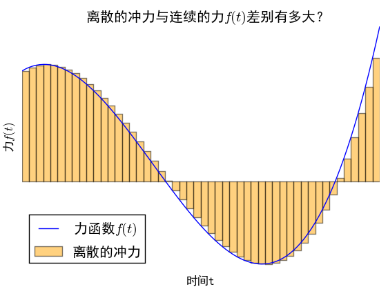Discretization of a force]

Of course, this was just a childhood flight of fancy on my part, and the reader shouldn't take it too seriously. But what does this puzzle have to do with the topic at hand? When studying vibration problems, we often encounter forced vibration under a time-varying force. Suppose the varying force is a known function of time, say $f(t)$. Even though we know the explicit form of $f(t)$, the motion under this external force is not necessarily easy to solve for, owing to the nonlinearity of $f$. However, if we could split a varying force into infinitely many constant forces (impulses) each acting over an infinitesimal time interval, then we could analyze the motion piecewise—and generally speaking, problems with constant forces are much easier than those with varying forces. If we discretize a varying force and then take the limit, should the result be the same as the motion under the original continuous varying force? This carries the same flavor as the puzzle at the start of the article: is the limit of a discretized process equivalent to the continuous process itself?

What's delightful is that in ordinary physical systems, splitting a force into constant forces over infinitely many small intervals does in fact lead to the correct answer—and this is precisely the Green's function method for linear ordinary differential equations. Let's work through this approach below. more

A First-Order Ordinary Differential Equation

As a first simple example, let's solve

$$\frac{dx(t)}{dt}+x(t)=f(t)$$

This is of course a simple ordinary differential equation, and we could use the method of variation of parameters. But let's set that method aside for now and instead re-derive the equation from a more physical viewpoint. When $f(t)\equiv 0$, the equation is easy to solve; and when $f(t)$ is a nonzero constant, it's also not hard to solve—we just add a constant to the original solution. But when $f(t)$ is a general function, solving becomes more involved. Suppose we already know the state $x(t)$ at time $t$, and we try to derive the state $x(t+\varepsilon)$ at time $t+\varepsilon$. Here $\varepsilon$ is a very small time interval, so small that $f(t)$ barely changes over it, so over the interval $[t,t+\varepsilon]$ we treat the external force as the constant $f(t)$. Then we have

$$\frac{d x(t+s)}{ds}+x(t+s)=f(t),\quad 0\leq s\leq \varepsilon$$

whose general solution is

$$x(t+s)=C e^{-t-s}+f(t)$$

and since at $s=0$ we have $x(t)=C e^{-t}+f(t)$, it follows that $C=[x(t)-f(t)]e^t$, giving us

$$x(t+s)=[x(t)-f(t)]e^{-s}+f(t)$$

and thus

$$\begin{aligned}x(t+\varepsilon)=&[x(t)-f(t)]e^{-\varepsilon}+f(t)\\ =&x(t)e^{-\varepsilon}+(1-e^{-\varepsilon})f(t)\\ =&x(t)(1-\varepsilon)+\varepsilon f(t)\end{aligned}$$

Of course, this step is quite trivial—we could get this result directly from the original differential equation, since we only care about first-order infinitesimals, so

$$\frac{x(t+\varepsilon)-x(t)}{\varepsilon}\approx\frac{dx(t)}{dt}=-x(t)+f(t)$$

A little rearrangement gives $x(t+\varepsilon)=x(t)(1-\varepsilon)+f(t)\varepsilon$, which is equivalent to the original equation. But going through the argument above lends our approach a clear physical meaning, so it's worth taking this slightly longer route.

Notice the character of this solution: starting from the state $x(t)$ at time $t$, we obtain the state at time $t+\varepsilon$; iterating this $n$ times, we can obtain the state at time $t+n\varepsilon$:

$$\begin{aligned}x(t+n\varepsilon)=&x(t+(n-1)\varepsilon)e^{-\varepsilon}+f(t+(n-1)\varepsilon)\varepsilon\\ =&[x(t+(n-2)\varepsilon)e^{-\varepsilon}+f(t+(n-2)\varepsilon)\varepsilon] e^{-\varepsilon}+f(t+(n-1)\varepsilon)\varepsilon\\ =&x(t+(n-2)\varepsilon)e^{-2\varepsilon}+ [e^{-\varepsilon}f(t+(n-2)\varepsilon)+f(t+(n-1)\varepsilon)]\varepsilon\\ =&\dots\\ =&x(t)e^{-n\varepsilon}+\varepsilon\sum_{i=1}^n e^{-(i-1)\varepsilon}f(t+n\varepsilon-i\varepsilon)\end{aligned}$$

Fixing $n\varepsilon=\tau$ and letting $n\to\infty$, we get

$$\begin{aligned}x(t+\tau)=&x(t)e^{-\tau}+\int_0^\tau e^{-s}f(t+\tau-s)ds\\ =&x(t)e^{-\tau}-\int_t^{t+\tau} e^{-t-\tau+s}f(s)ds\end{aligned}$$

This gives us the (exact) solution at time $t+\tau$: substituting in any known initial state, we can obtain the state at any subsequent time. Here

$$G(t,s)=e^{-t+s}$$

is called the Green's function of the system; with it we can obtain $x(t)$ from $x(s)$.

A Second-Order Ordinary Differential Equation

The first-order case is too trivial for us to appreciate the value of this approach. Let's now apply the same idea to derive the Green's function solution of

$$\frac{d^2 x(t)}{dt}+x(t)=f(t)$$

Unlike the first-order case, the increase in order turns the derivation into matrix and vector operations. This equation is equivalent to the system

$$\frac{d}{dt}\begin{pmatrix} x(t)\\ x'(t)\end{pmatrix}=\begin{pmatrix} 0&1\\ -1&0 \end{pmatrix}\begin{pmatrix} x(t)\\ x'(t)\end{pmatrix}+\begin{pmatrix} 0\\ f(t)\end{pmatrix}$$

that is,

$$\begin{pmatrix} x(t+\varepsilon)\\x'(t+\varepsilon)\end{pmatrix}=\left[I+\varepsilon\begin{pmatrix} 0&1\\ -1&0 \end{pmatrix}\right]\begin{pmatrix} x(t)\\ x'(t)\end{pmatrix}+\varepsilon\begin{pmatrix} 0\\ f(t)\end{pmatrix}$$

This is the recursion formula over an infinitesimal interval. Note that we obtained this equation directly from the original equation. Of course, we could also mimic the more physically-motivated derivation used in the first-order case to arrive at essentially the same equation (differing at most by terms of order $\varepsilon^2$). But however we arrive at this equation, we know its physical meaning is exactly as in the first-order case: decomposing the varying force into infinitely many constant forces, each acting over a small time interval.

Iterating the above equation $n$ times gives

$$\begin{aligned}\begin{pmatrix} x(t+n\varepsilon)\\x'(t+n\varepsilon)\end{pmatrix}=&\left[I+\varepsilon\begin{pmatrix} 0&1\\ -1&0 \end{pmatrix}\right]^n\begin{pmatrix} x(t)\\ x'(t)\end{pmatrix}\\&+\varepsilon\sum_{i=1}^{n}\left[I+\varepsilon\begin{pmatrix} 0&1\\ -1&0 \end{pmatrix}\right]^{n-i}\begin{pmatrix} 0\\ f(t+n\varepsilon-i\varepsilon)\end{pmatrix}\end{aligned}$$

Again letting $\tau=n\varepsilon$, fixing $\tau$, and letting $n\to\infty$, we obtain

$$\begin{aligned}\begin{pmatrix} x(t+\tau)\\x'(t+\tau)\end{pmatrix}=&\exp \left[\begin{pmatrix} 0&1\\ -1&0 \end{pmatrix}\tau\right]\begin{pmatrix} x(t)\\ x'(t)\end{pmatrix}\\&+\int_0^{\tau}ds\exp\left[\begin{pmatrix} 0&1\\ -1&0 \end{pmatrix}(\tau-s)\right]\begin{pmatrix} 0\\ f(t+\tau-s)\end{pmatrix}\end{aligned}$$

Notice that

$$\begin{pmatrix} 0&1\\ -1&0 \end{pmatrix}^4=I$$

That is, this matrix has a periodicity similar to that of the imaginary unit $i$—it plays the same role among second-order matrices that $i$ plays among complex numbers. So, by Euler's formula, we can immediately write

$$\exp \left[\begin{pmatrix} 0&1\\ -1&0 \end{pmatrix}\tau\right]=I \cos \tau+\begin{pmatrix} 0&1\\ -1&0 \end{pmatrix}\sin\tau$$

Substituting this in gives

$$\begin{aligned}\begin{pmatrix} x(t+\tau)\\x'(t+\tau)\end{pmatrix}=&\begin{pmatrix} x(t)\\ x'(t)\end{pmatrix}\cos\tau+\begin{pmatrix} x'(t)\\ -x(t)\end{pmatrix}\sin\tau\\&+\int_0^{\tau}ds\begin{pmatrix} 0\\ f(t+\tau-s)\end{pmatrix}\cos\left(\tau-s\right)\\&+\int_0^{\tau}ds\begin{pmatrix} f(t+\tau-s)\\0 \end{pmatrix}\sin\left(\tau-s\right)\end{aligned}$$

that is,

$$\begin{aligned}x(t+\tau)=&x(t)\cos\tau+x'(t)\sin\tau+\int_0^{\tau}f(t+\tau-s)\sin(\tau-s)ds\\ =&x(t)\cos\tau+x'(t)\sin\tau-\int_t^{t+\tau}f(s)\sin(s-t)ds\end{aligned}$$

and

$$x'(t+\tau)=x'(t)\cos\tau-x(t)\sin\tau-\int_t^{t+\tau}f(s)\cos(s-t)ds$$

The Feynman Lectures on Physics

It may come as a surprise to the reader that the idea above comes from Feynman's Lectures on Physics! It appears in the latter half of §25-2 of Volume I.

I don't know whether other textbooks present this idea, but as far as I'm concerned, I only recently learned it from Feynman—and it really was an eye-opening, "aha" moment! With such a clear physical meaning, how could this not be more widely known among math and physics enthusiasts! Back when I was reading textbooks on ordinary differential equations and came across the Green's function method, I would simply skip over it, because the Green's function for ODEs never seemed to carry as obvious a meaning as the Green's function for PDEs. I could barely memorize it without understanding what it meant. Now, thanks to Feynman's "guidance," I finally have a crystal-clear understanding of the Green's function method for ODEs! And note—this clarity came from a physics lecture book!

It must be said: no matter how one reads Feynman himself, or his works, it is never too much.