Describing Rotations in Three-Dimensional Space with Matrices

矩阵描述三维空间旋转 苏剑林 · 2013-12-28 · Mathematics rotation matrix 3D quaternion

This section gives a brief introduction to describing rotations using matrices. In the two-dimensional plane, complex numbers are undoubtedly the best tool for describing rotations; however, when we generalize to three-dimensional space, we need to bring in "quaternions." In order to prove results about quaternions, we first need a matrix description of three-dimensional rotations. The most general rotational motion is: rotation by an angle $\theta$ about some axis. This means we need three parameters to describe it: at least two parameters to pin down an axis, and one parameter to specify the angle. Therefore, if we wanted to use "numbers" to describe scaling and rotation in three-dimensional space, "three-part numbers" would clearly not suffice — accomplishing this requires at least four components. This is yet another angle from which we see why three-component number systems cannot exist.

The matrix approach

First, we recognize that if the rotation axis happens to be one of the coordinate axes, the rotation matrix takes its simplest form. For instance, the coordinates of a vector $\boldsymbol{x}=(x_0,y_0,z_0)^{T}$ after rotating counterclockwise by angle $\theta$ about the $z$-axis can be written as

$$\begin{equation} \boldsymbol{R}_{\theta}\boldsymbol{x}\end{equation}$$

where

$$\begin{equation}\label{xuanzhuanjuzhen} \boldsymbol{R}_{\theta}=\left[ \begin{array}{\cdot {20}{c}} \cos\theta&{ - \sin\theta}&0\\ \sin\theta & \cos\theta &0\\ 0&0&1 \end{array} \right] \end{equation}$$

If the rotation axis is not a coordinate axis but is instead determined by a unit column vector $\boldsymbol{u}=(x_1,y_1,z_1)$, this simultaneously determines a plane perpendicular to $\boldsymbol{u}$. Within that plane we can find two orthogonal unit column vectors $\boldsymbol{e}_1,\boldsymbol{e}_2$, and together with $\boldsymbol{e}_1,\boldsymbol{e}_2,\boldsymbol{u}$ we can build a new right-handed Cartesian coordinate system. Suppose that, in this new coordinate system, the coordinates of the original vector $\boldsymbol{x}$ are $\boldsymbol{\xi}=(\xi_1,\xi_2,\xi_3)^T$; then

$$\begin{equation} \left[ \boldsymbol{e}_1,\boldsymbol{e}_2,\boldsymbol{u} \right] \boldsymbol{\xi}=\boldsymbol{x} \end{equation}$$

Describing the rotation is convenient in the new coordinate system — it is simply the matrix $\eqref{xuanzhuanjuzhen}$. After rotating counterclockwise by angle $\theta$ about the $\boldsymbol{u}$-axis, the coordinates become

$$\begin{equation} \boldsymbol{R}_{\theta} \boldsymbol{\xi}=\boldsymbol{R}_{\theta}\left[ \boldsymbol{e}_1,\boldsymbol{e}_2,\boldsymbol{u} \right]^{-1}\boldsymbol{x} \end{equation}$$

The above are the coordinates in the $\boldsymbol{e}_1,\boldsymbol{e}_2,\boldsymbol{u}$ coordinate system. Converting back to our original Cartesian coordinate system gives

$$\begin{equation}\label{xuanzhuan} \left[ \boldsymbol{e}_1,\boldsymbol{e}_2,\boldsymbol{u} \right]\boldsymbol{R}_{\theta}\left[ \boldsymbol{e}_1,\boldsymbol{e}_2,\boldsymbol{u} \right]^{-1}\boldsymbol{x} \end{equation}$$

Equation $\eqref{xuanzhuan}$ gives the coordinates after rotation. It describes the most general rotation in three-dimensional space. Note that the matrix $\left[ \boldsymbol{e}_1,\boldsymbol{e}_2,\boldsymbol{u} \right]$ is orthogonal, so its inverse is simply $\left[ \boldsymbol{e}_1,\boldsymbol{e}_2,\boldsymbol{u} \right]^{-1}=\left[ \begin{array}{*{20}{c}}\boldsymbol{e}_1^T \\ \boldsymbol{e}_2^T \\ \boldsymbol{u}^{T}\end{array} \right]$, and hence the coordinates after rotation are

$$\begin{equation}\label{xuanzhuanzuobiao3} \left[ \boldsymbol{e}_1,\boldsymbol{e}_2,\boldsymbol{u} \right]\boldsymbol{R}_{\theta}\left[ \begin{array}{\cdot {20}{c}}\boldsymbol{e}_1^T \\ \boldsymbol{e}_2^T \\ \boldsymbol{u}\end{array}\right]\boldsymbol{x} =\left[ \boldsymbol{e}_1,\boldsymbol{e}_2,\boldsymbol{u} \right]\boldsymbol{R}_{\theta}\left[ \begin{array}{\cdot {20}{c}}\boldsymbol{e}_1 \cdot \boldsymbol{x} \\ \boldsymbol{e}_2 \cdot \boldsymbol{x}\\ \boldsymbol{u} \cdot \boldsymbol{x}\end{array} \right] \end{equation}$$

What remains is determining $\boldsymbol{e}_1,\boldsymbol{e_2}$. If it is not easy to quickly find two vectors satisfying the required conditions, we can make use of the cross product:

$$\begin{equation}\label{chaji} \boldsymbol{e}_1=\frac{\boldsymbol{u}\times\boldsymbol{x}}{|\boldsymbol{u}\times\boldsymbol{x}|},\boldsymbol{e}_2=\frac{\boldsymbol{u}\times(\boldsymbol{u}\times\boldsymbol{x})}{|\boldsymbol{u}\times(\boldsymbol{u}\times\boldsymbol{x})|}=\frac{(\boldsymbol{u}\cdot\boldsymbol{x})\boldsymbol{u}- \boldsymbol{x}}{|\boldsymbol{u}\times\boldsymbol{x}|} \end{equation}$$

The advantage of the cross product is obvious: substituting $\eqref{chaji}$ into $\eqref{xuanzhuanzuobiao3}$ gives

$$\begin{equation}\label{juzhenxuanzhuanhuajian} \begin{aligned} &\left[ \frac{\boldsymbol{u}\times\boldsymbol{x}}{|\boldsymbol{u}\times\boldsymbol{x}|},\frac{(\boldsymbol{u}\cdot\boldsymbol{x})\boldsymbol{u}- \boldsymbol{x}}{|\boldsymbol{u}\times\boldsymbol{x}|},\boldsymbol{u} \right]\boldsymbol{R}_{\theta}\left[ \begin{array}{\cdot {20}{c}}0 \\ \frac{(\boldsymbol{u} \cdot \boldsymbol{x})^2-\boldsymbol{x}^2}{|\boldsymbol{u}\times\boldsymbol{x}|}\\ \boldsymbol{u} \cdot \boldsymbol{x}\end{array} \right]\\ =&\left[ \frac{\boldsymbol{u}\times\boldsymbol{x}}{|\boldsymbol{u}\times\boldsymbol{x}|},\frac{(\boldsymbol{u}\cdot\boldsymbol{x})\boldsymbol{u}- \boldsymbol{x}}{|\boldsymbol{u}\times\boldsymbol{x}|},\boldsymbol{u} \right]\left[ \begin{array}{\cdot {20}{c}} |\boldsymbol{u}\times \boldsymbol{x}| \sin\theta \\ -|\boldsymbol{u}\times \boldsymbol{x}|\cos\theta \\ \boldsymbol{u} \cdot \boldsymbol{x}\end{array} \right]\\ =&\left(\boldsymbol{u}\times\boldsymbol{x} \right)\sin\theta-\left[(\boldsymbol{u}\cdot\boldsymbol{x})\boldsymbol{u}- \boldsymbol{x}\right]\cos\theta+(\boldsymbol{u}\cdot\boldsymbol{x})\boldsymbol{u}\\ =&\left(\boldsymbol{u}\times\boldsymbol{x} \right)\sin\theta+\left[(\boldsymbol{u}\times\boldsymbol{x})\times\boldsymbol{u}\right]\cos\theta+(\boldsymbol{u}\cdot\boldsymbol{x})\boldsymbol{u} \end{aligned} \end{equation}$$

This is known as Rodrigues' rotation formula, and it is the simplest form for describing a three-dimensional rotation using vectors. It is written in this final form because it has a clear geometric meaning — indeed, one can derive this final expression in $\eqref{juzhenxuanzhuanhuajian}$ entirely without matrix analysis, using only geometric arguments and the vector cross product. Moreover, if $\boldsymbol{x} \perp \boldsymbol{u}$ (a condition that, in practice, is not particularly restrictive), the coordinate rotation formula becomes considerably simpler:

$$\begin{equation} (\boldsymbol{u}\times\boldsymbol{x})\sin\theta +\boldsymbol{x}\cos\theta \end{equation}$$

The geometric approach

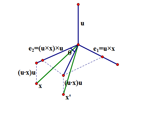Diagram of rotation]]

Suppose the unit vector $\boldsymbol{u}$ is the rotation axis, and we want to find the coordinates of a vector $\boldsymbol{x}$ after it is rotated counterclockwise by angle $\theta$ about the axis $\boldsymbol{u}$. We take the cross product $\boldsymbol{e}_1=\boldsymbol{u}\times\boldsymbol{x}$ of $\boldsymbol{u}$ and $\boldsymbol{x}$, obtaining a vector perpendicular to both $\boldsymbol{u}$ and $\boldsymbol{x}$; then we take a further cross product $\boldsymbol{e}_2=(\boldsymbol{u}\times\boldsymbol{x})\times\boldsymbol{u}$, obtaining a vector coplanar with $\boldsymbol{u}$, $\boldsymbol{x}$, and $\boldsymbol{u}$, which has the same length as $\boldsymbol{u}\times\boldsymbol{x}$ and is perpendicular to both $\boldsymbol{u}$ and $\boldsymbol{u}\times\boldsymbol{x}$.

Notice that

$$(\boldsymbol{u}\times\boldsymbol{x})\times\boldsymbol{u}=\boldsymbol{x}-(\boldsymbol{u}\cdot\boldsymbol{x})\boldsymbol{u}$$

In other words, the projection of the vector $\boldsymbol{x}$ onto the plane $\boldsymbol{e}_1 ,\boldsymbol{e}_2$ is precisely $\boldsymbol{e}_2$, while its projection onto the $\boldsymbol{u}$-axis is $(\boldsymbol{u}\cdot\boldsymbol{x})\boldsymbol{u}$. Note that during the rotation, only the component lying in the $\boldsymbol{e}_1 ,\boldsymbol{e}_2$ plane — that is, the plane of rotation — changes. Describing the transformation within the rotation plane is straightforward; it is simply

$$\boldsymbol{e}_2 \cos\theta +\boldsymbol{e}_1\sin\theta$$

Adding back the component $(\boldsymbol{u}\cdot\boldsymbol{x})\boldsymbol{u}$ along the $\boldsymbol{u}$-axis gives us the coordinates after rotation, namely

$$\left(\boldsymbol{u}\times\boldsymbol{x} \right)\sin\theta+\left[(\boldsymbol{u}\times\boldsymbol{x})\times\boldsymbol{u}\right]\cos\theta+(\boldsymbol{u}\cdot\boldsymbol{x})\boldsymbol{u}$$

In this way we have arrived once again at $\eqref{juzhenxuanzhuanhuajian}$.