*Rethinking Matrices, Part 2*: What Is a Matrix?
In the previous post I described my understanding of matrices purely from the point of view of algebraic operations. As we saw, once we equip matrices with the appropriate rules of operation, they turn out to be enormously useful in algebra, analysis, and beyond. But pure algebra alone is not enough. To make the picture complete, it is best to find a matching geometric object, since only then can we grasp matrices intuitively and use them with real fluency.
A Geometric Understanding
I'll assume the reader has already read Meng Yan's three-part series Understanding Matrices, so I won't repeat all the details here. As we know, the matrix A
$$\begin{pmatrix}a_{11} & a_{12} \\ a_{21} & a_{22}\end{pmatrix}$$
is in fact made up of two vectors $[a_{11},a_{21}]^T$ and $[a_{12},a_{22}]^T$ (here vectors are always taken to be column vectors), and together they describe a planar (affine) coordinate system. In other words, these two vectors are actually the two basis vectors of that coordinate system, and the operation $y=Ax$ tells us: given a vector x expressed in the $A$ coordinate system, what does it look like in the $I$ coordinate system? Here the $I$ coordinate system is simply our usual rectangular coordinate system — that is, any vector (including the vectors that make up a matrix), as long as no matrix is applied to it beforehand, is understood to be measured in rectangular coordinates.more
(In fact, the identity matrix I represents the default rectangular coordinate system — though this statement does not always hold in general, for now we are seeking an intuitive picture, so let's work with the simplest case.)
Too many words rarely clarify a point like this, so let's use a picture to explain:
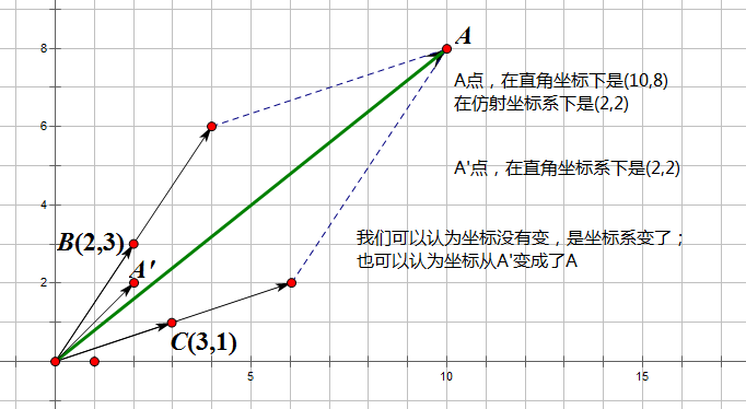 Geometric meaning of a matrix
The matrix A used in the figure is
[3,2]
[1,3]
This defines an affine coordinate system. In this coordinate system there is a vector $x=[2,2]^T$, whose coordinates measured in the rectangular coordinate system are $[10,8]^T$. Now it isn't hard to see that if we simply carry out the matrix multiplication, we get
$$Ax=[3\cdot 2+2\cdot 2,1\cdot 2+3\cdot 2]^T=[10,8]^T$$
exactly what we expected!
Why does this property hold? Actually it stems directly from how we define matrix multiplication. Conversely, if we were to define matrix multiplication via this geometric picture, we would recover exactly the matrix-multiplication formula we learned from textbooks. Higher-order matrices can be treated by the same analogy. The derivation is a simple exercise — why not try working it out yourself?
Now we come back to the point Meng Yan makes in his article: when a matrix acts on a vector (corresponding to a point), we can either think of the point as staying fixed while the coordinate system changes from rectangular to affine, or we can think of the matrix as "moving" (transforming) a point A′ in the rectangular coordinate system to the point A. Both descriptions work, exactly as Meng Yan says: "motion is relative." To put it more precisely, both descriptions need to be held in mind together for the best understanding. A matrix is a transformation from one point to another, and the way this transformation is carried out is precisely a change of coordinate system.
Of course, the discussion above only covers matrix-times-vector multiplication. What about matrix-times-matrix multiplication? Take $AB$, for example: we can think of the matrix $B$ as specifying a coordinate system, but the components of this coordinate system are measured within the $A$ coordinate system, while $A$ itself is measured in the rectangular coordinate system. So we need to multiply each component (column vector) of $B$ by the matrix A in order to obtain the "image" of this affine coordinate system as seen in rectangular coordinates. This directly gives us the formula for matrix multiplication, and it also clearly answers the question of "why can an n×n matrix only be meaningfully multiplied by another n×n matrix" — because the two must be measured within the same space for the measurement to be completely and uniquely determined. In the same way, it makes no sense to discuss n vectors of dimension n within an (n+1)-dimensional space, because to an observer in that (n+1)-dimensional space, those vectors merely span a "surface," and the extra dimension is free to vary arbitrarily; and discussing (n+1)-dimensional vectors within an n-dimensional space makes even less sense, since there simply aren't enough dimensions to go around.
With this intuitive geometric picture in hand, many questions become almost self-evident — for instance, questions about determinants, similar matrices, and so on, which we'll get to next time.
A Brief Introduction to Tensors
We've already seen, roughly speaking, that an ordered collection of numbers gives rise to a vector, and an ordered collection of vectors gives rise to a matrix. Each of these newly constructed objects is more powerful than the last. So naturally one might wonder: could an ordered collection of matrices produce a "cube array," and would it be even more powerful? More generally, what about an n-dimensional cube array? This line of thinking is well-founded — there is indeed such an object studied in mathematics, and it is called a tensor.
Put most simply, an order-n tensor is an n-dimensional cube array, so an order-0 tensor corresponds to a single number, while vectors and matrices correspond to order-1 and order-2 tensors respectively; what we call a three-dimensional cube array is an order-3 tensor. Of course, tensors belong to a very deep branch of mathematics, and their properties and uses can't possibly be explained so simply. Recall that it was Einstein who used tensor analysis as the mathematical tool for building his magnificent general theory of relativity. If the opportunity arises, we will certainly return to this topic.
For now, though, let's go back to matrices and talk about the determinant of a matrix.
Translated automatically with claude-sonnet-5; all equations are reproduced verbatim from the source. Copyright remains with the original author.