An "Unsolved Mystery": Why Is the Midpoint Rectangle Rule Never Taught?
Foreword
In some earlier posts, we've already pointed out several flaws in current textbooks — things like getting priorities backwards (the most obvious case being those linear algebra textbooks that dive straight into systems of linear equations), a lack of intuition, and a lack of pedagogical guidance. I suspect the main reason behind these problems is simply following the crowd too closely: everyone writes their textbook the way everyone else does, without their own perspective or logic, and so certain common flaws just get passed down generation after generation. Perhaps that's exactly why we end up with such a strange phenomenon: there exists a method that requires less computation and is actually more accurate, yet textbooks almost never mention it — while another method, one that requires slightly more computation and is slightly less accurate, gets taught in practically every textbook of the same kind. This can only be called an "unsolved mystery"...
This post is about exactly such a pair of methods, used for approximating definite integrals: the "midpoint rectangle rule" and the "trapezoidal rule." I imagine most people who've studied calculus will remember the latter — it's the method that shows up in nearly every calculus textbook. The former, I suspect, many readers have never even heard of. Yet, surprisingly, it requires slightly less computation while achieving slightly higher accuracy. This post will introduce both methods and compare their precision. What makes this post a bit different is that the proof follows the approach used in Visual Complex Analysis, giving a beautiful geometric way to estimate the error!
Our goal is to approximate $\int_a^b f(x)dx$ in cases where it's hard to compute exactly. These methods are all, at their core, based on the idea that an integral is an area.
Two Different Methods
The idea behind the trapezoidal rule is quite simple. As shown in the figure, we divide the interval [a,b] into n equal parts, each of length h (equal partitioning isn't strictly required, but it does simplify the computation). We then connect the points $f(a),f(x_1),...,f(x_{n-1}),f(b)$ in sequence, forming n trapezoids. Adding up the areas of these n trapezoids gives us an approximation of $\int_a^b f(x)dx$. This gives us the following result:
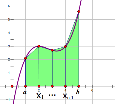 Trapezoidal Rule
$$\begin{aligned}\int_a^b f(x)dx \approx \frac{f(a)+f(x_1)}{2}\cdot h+\frac{f(x_1)+f(x_2)}{2}\cdot h+...+\frac{f(x_{n-1})+f(b)}{2}\cdot h \\ =[\frac{f(a)+f(b)}{2}+\sum_{i=1}^{n-1}f(x_i)]\cdot h\end{aligned}\tag{1}$$
Intuition tells us that the larger the number of subdivisions n (i.e., the smaller h), the smaller the error. We'll get into the detailed error analysis later. For now, let's look at another method for approximating a definite integral — the midpoint rectangle rule.
Its idea seems even more straightforward. We again divide [a,b] into n equal parts of length h. Then, for each subinterval, we evaluate f(x) at its midpoint, and construct a rectangle of height f(x) and width h over that subinterval. Finally, we sum up the areas of all these rectangles. This gives us the following formula:
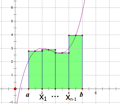 Midpoint Rectangle Rule
$$\begin{aligned}\int_a^b f(x)dx \approx f(\frac{a+x_1}{2})\cdot h+f(\frac{x_1+x_2}{2})\cdot h+...+f(\frac{x_{n-1}+b}{2})\cdot h \\ =[f(\frac{a+x_1}{2})+f(\frac{x_1+x_2}{2})+...+f(\frac{x_{n-1}+b}{2})]h\end{aligned}\tag{2}$$
In terms of computational cost, formula (1) requires evaluating f(x) at (n+1) nodes, while formula (2) only requires evaluating n nodes. Just from this alone, formula (2) already has a slight edge. So how do their respective accuracies compare? Here's where a wonderful geometric argument comes in...
Error Analysis
 Error Analysis
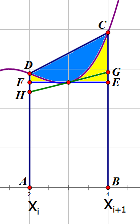
Let's "break the whole into parts" and study the error on a single small subinterval in isolation. We choose h small enough that the little piece of curve within this subinterval has a single, consistent type of curvature (either convex or concave throughout). The figure illustrates both the trapezoidal rule and the midpoint rectangle rule.
The error given by the trapezoidal rule is the area enclosed between line DC and the curve (the blue region), while the error given by the midpoint rectangle rule is the area enclosed between line EF and the curve (the yellow region). At a glance, it's clear that the blue area looks larger than the yellow area, which intuitively suggests that the trapezoidal rule has a larger error. Of course, we can't rely on impressions alone — we need to prove this more rigorously. From the figure it's easy to see that the trapezoidal estimate is larger than the true value (though this is only true for the particular case shown here), but the midpoint rectangle case is less obvious, since the horizontal line EF at the midpoint isn't necessarily tangent to the curve — it might actually intersect the curve. A brilliant trick here is to rotate EF about the midpoint until it becomes tangent to the curve, giving line GH. After this rotation, rectangle ABEF becomes trapezoid ABGH, and clearly the area is unchanged. So it's easy to see that trapezoid ABGH has smaller area than the region under the original curve — meaning the midpoint rectangle estimate is also larger than the true value.
In fact, in the general case, the true value of the definite integral is sandwiched between the results given by the trapezoidal rule and the midpoint rectangle rule.
This tells us that the maximum error of both methods can't exceed the area of quadrilateral CDHG, so what we need to do is find the relationship between this area and h. When h is very small, we can treat the original curve as approximately a circular arc, and then rotate the whole figure so that line GH lies horizontally. Let $|GH|=a$, and since h is proportional to |GH|, the two are interchangeable to some degree.
 Approximating Arc
At this point, quadrilateral CDHG can be approximately treated as a rectangle, with area $\Delta S=|GH|*|PQ|$, while $|DP|^2=|OP|*|PQ|$.
Therefore $\Delta S=\frac{|GH|^3}{4|OP|}\propto |GH|^3 \propto h^3$
Here we've only computed the error for a single subinterval. Since the total error requires summing these errors over all subintervals, the total error is $\Delta \propto h^2$
Theoretical analysis actually tells us that the errors of both methods are indeed of the same order, $h^2$. But how do their relative errors compare? We need to compute the ratio of the blue area (S1) to the yellow area (S2).
$$\begin{aligned}S_1=r^2 \theta-r \cos\theta\cdot r \sin\theta=r^2 \theta-\frac{1}{2} r^2 \sin2\theta \\ S_2=2r \sin\theta\cdot r(1-\cos\theta)-(r^2 \theta-\frac{1}{2} r^2 \sin2\theta)=2r^2 \sin\theta-r^2 \theta-\frac{1}{2} r^2 \sin2\theta\end{aligned}$$
Expanding via Taylor series to third order gives
$$\begin{aligned}S_1 \approx \frac{4\theta^3}{3} \\ S_2 \approx \frac{2\theta^3}{3}\end{aligned}$$
In other words, the error of the trapezoidal rule is twice that of the midpoint rectangle rule!
Afterword
Actually, the main point of this post was to introduce the midpoint rectangle rule to readers, and to share the beautiful geometric proof technique from Visual Complex Analysis — not to criticize textbooks per se. In my view, the midpoint rectangle rule is a genuinely good method, and what's puzzling is that textbooks simply never mention it — it was thanks to this complex analysis book that I even learned about it. But this does serve as a reminder that, when reading, we should keep asking "why," and also keep asking "what other ways might there be?" We shouldn't blindly trust the authority of a textbook, because in the end, only knowledge itself is the real authority. Indeed, after finishing this post, you should also read it again with a critical eye. ^_^
I also want to give a shout-out to Visual Complex Analysis. It presents complex analysis in a way that's completely different from typical textbooks — emphasizing geometric applications, emphasizing intuition, and paying close attention to connections with physics. This is exactly what a complex analysis textbook should do. Reading it carefully has taught me a great deal. I've only gotten through a few pages so far, but I've already decided to make it my personal standard reference for complex analysis!
Translated automatically with claude-sonnet-5; all equations are reproduced verbatim from the source. Copyright remains with the original author.