Asymptotic Estimate of the Maximum of n Normal Random Numbers

n个正态随机数的最大值的渐近估计 苏剑林 · 2025-11-06 · Mathematics probability approximation random estimation

Let $z_1,z_2,\cdots,z_n$ be $n$ random numbers sampled i.i.d. from the standard normal distribution. From these we can construct many derived random variables — for instance $z_1+z_2+\cdots+z_n$, which is still normally distributed, or $z_1^2+z_2^2+\cdots+z_n^2$, which follows a chi-squared distribution. In this post we care about the distribution of their maximum $z_{\max} = \max\{z_1,z_2,\cdots,z_n\}$, and in particular its expectation $\mathbb{E}[z_{\max}]$.

The conclusion first

The basic estimate for $\mathbb{E}[z_{\max}]$ is:

Let $z_1,z_2,\cdots,z_n\sim\mathcal{N}(0,1)$, $z_{\max} = \max\{z_1,z_2,\cdots,z_n\}$, then
\begin{equation}\mathbb{E}[z_{\max}]\sim \sqrt{2\log n}\label{eq:E-z-max}\end{equation}

Here, the meaning of $\sim$ in equation $\eqref{eq:E-z-max}$ is:

\begin{equation}\lim_{n\to\infty} \frac{\mathbb{E}[z_{\max}]}{\sqrt{2\log n}} = 1\end{equation}

From this we can see that as $n$ grows, this result becomes relatively more and more accurate. A sharper result is:

\begin{equation}\mathbb{E}[z_{\max}]\sim \sqrt{2\log \frac{n}{\sqrt{2\pi}}}\end{equation}

We can verify these with NumPy:

import numpy as np

n = 4096
z = np.random.randn(10000, n)
E_z_max = z.max(axis=1).mean()  # ≈ 3.63
approx1 = np.sqrt(2 * np.log(n))  # ≈ 4.08
approx2 = np.sqrt(2 * np.log(n / np.sqrt(2 * np.pi)))  # ≈ 3.85

A quick upper bound

This post gives three proofs of the above conclusion. The first proof comes from the answer by @Sivaraman] in the thread Expectation of the maximum of gaussian random variables]. Strictly speaking it only proves $\mathbb{E}[z_{\max}] \leq \sqrt{2\log n}$, but the proof itself is quite elegant and worth studying.

The proof cleverly exploits the convexity of $\exp$: for any $t > 0$, we can write

\begin{equation}\exp(t\mathbb{E}[z_{\max}]) \leq \mathbb{E}[\exp(t z_{\max})] = \mathbb{E}[\max_i \exp(t z_i)]\leq \sum_{i=1}^n\mathbb{E}[\exp(t z_i)] = n \exp(t^2 / 2)\end{equation}

The first $\leq$ follows from Jensen's inequality, while the second $\leq$ comes from replacing the maximum with a sum. Now taking the logarithm of both sides and rearranging, we get

\begin{equation}\mathbb{E}[z_{\max}] \leq \frac{\log n}{t} + \frac{t}{2}\end{equation}

Note that this holds for any $t > 0$, so we can choose the $t$ that minimizes the right-hand side, giving the tightest approximation. By the basic inequality, the minimum of the right-hand side is attained at $t=\sqrt{2\log n}$; substituting this back gives

\begin{equation}\mathbb{E}[z_{\max}] \leq \sqrt{2\log n}\end{equation}

The distinguishing feature of this derivation is that it's simple and quick, requiring little extra background knowledge. However, in theory it only gives an upper bound — it just happens, surprisingly, to be quite accurate, and indeed matches the asymptotic result.

The standard approach

For those accustomed to deriving formulas step by step (such as the author), the derivation above has a somewhat "unorthodox" flavor to it, since the conventional approach would be to first find the probability density function of $z_{\max}$ and then compute the expectation via integration. In this section we follow that route.

Probability density

For 1-dimensional distributions, the probability density function and the cumulative distribution function are two sides of the same coin, and to find the probability density of $z_{\max}$ we need the cumulative distribution function to help. The probability density of the standard normal distribution is $p(z)=\exp(-z^2/2)/\sqrt{2\pi}$, and its cumulative distribution function $\Phi(z)=\int_{-\infty}^z p(x)dx$ — a non-elementary function — represents the probability that the random variable is less than or equal to $z$.

To find the cumulative distribution function of $z_{\max}$, i.e. $P(z_{\max} \leq z)$, note that $z_{\max} \leq z$ is equivalent to $z_1 \leq z, z_2\leq z, \cdots, z_n\leq z$ holding simultaneously. Since $z_i$ are sampled independently, the probability that they all hold simultaneously equals the product of their individual probabilities:

\begin{equation}P(z_{\max} \leq z) = \prod_{i=1}^n P(z_i \leq z) = [\Phi(z)]^n \end{equation}

So the cumulative distribution function of $z_{\max}$ is simply $[\Phi(z)]^n$ — a very clean result. Note that we haven't yet used the assumption that $z$ is normally distributed, so this is in fact a general result: for $n$ numbers sampled i.i.d. from any distribution, the cumulative distribution function of their maximum is the $n$-th power of the original distribution's cumulative distribution function. Differentiating this now gives the probability density function $p_{\max}(z)$ of $z_{\max}$:

\begin{equation}p_{\max}(z) = n[\Phi(z)]^{n-1} p(z) \end{equation}

When $n=50,100,200$, the plot of $p_{\max}(z)$ looks like this:

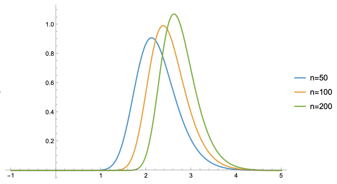Plot of p_max(z) for several different values of n

Laplace's method

With the probability density function in hand, we can in principle compute the expectation by integration:

\begin{equation}\mathbb{E}[z_{\max}] = \int_{-\infty}^{\infty} z\, p_{\max}(z) dz\end{equation}

But clearly this integral is not easy to evaluate, so we need to look for some tractable approximation. From the plot above, we can see that the shape of $p_{\max}(z)$ actually also resembles an inverted-bell curve like the normal distribution, so it's natural to look for a normal-distribution approximation — this is called "Laplace approximation."

The first step in finding a normal approximation is to locate the maximum of the inverted-bell-shaped curve, and then expand $\log p_{\max}(z)$ to second order around that point. If our goal is merely to find the mean, then locating the maximum point suffices, since the mean of a normal distribution coincides with the location of the maximum of its density. To find this maximum point $z_*$, we first compute $\log p_{\max}(z)$:

\begin{equation}\begin{aligned} \log p_{\max}(z) =&\, \log n + (n-1)\log \Phi(z) + \log p(z) \\ =&\, \log n + (n-1)\log \Phi(z) - \frac{z^2}{2} - \frac{1}{2}\log 2\pi \end{aligned}\end{equation}

Differentiating with respect to $z$ gives

\begin{equation}\frac{d}{dz}\log p_{\max}(z) = (n-1) \frac{p(z)}{\Phi(z)} - z = \frac{(n-1)\exp(-z^2/2)}{\Phi(z) \sqrt{2\pi}} - z\end{equation}

Setting this equal to zero and rearranging, we obtain

\begin{equation}z_* = \sqrt{2\log\frac{n-1}{z_*\Phi(z_*)\sqrt{2\pi}}}\label{eq:z}\end{equation}

Approximate solution

The next task is to solve the equation $\eqref{eq:z}$. Of course we don't need an exact solution — an asymptotic estimate will do. Note that $z\Phi(z)$ already exceeds 1 once $z\geq 1.15$, and since we're after the asymptotic solution, we can naturally assume $z_* \geq 1.15$ holds, giving

\begin{equation}z_* < \sqrt{2\log\frac{n-1}{\sqrt{2\pi}}}\end{equation}

Substituting this result back into the equation $\eqref{eq:z}$, and using $\Phi(z) < 1$, we obtain

\begin{equation}z_* > \sqrt{2\log\frac{n-1}{\sqrt{2\log\frac{n-1}{\sqrt{2\pi}}}\sqrt{2\pi}}}\end{equation}

From these upper and lower bounds we get

\begin{equation}z_* \sim \sqrt{2\log\frac{n-1}{\sqrt{2\pi}}}\sim \sqrt{2\log\frac{n}{\sqrt{2\pi}}}\sim \sqrt{2\log n}\end{equation}

This is the asymptotic result we sought for $\mathbb{E}[z_{\max}]$. For further discussion of this problem, see the Fisher–Tippett–Gnedenko theorem] and the Generalized extreme value distribution].

Inverse-transform sampling

The final proof is based on the idea of inverse cumulative distribution function sampling: let the cumulative distribution function of a 1-dimensional distribution be $\Phi(z)$, with inverse function $\Phi^{-1}(z)$. Then one way to sample from this distribution is

\begin{equation}z = \Phi^{-1}(\varepsilon),\qquad \varepsilon\sim U(0,1)\end{equation}

That is, applying the inverse cumulative distribution function converts a uniform distribution into the target distribution. So if we sample $n$ points $z_1,z_2,\cdots,z_n$ from an arbitrary target distribution, this is equivalent to saying that $\Phi(z_1),\Phi(z_2),\cdots,\Phi(z_n)$ is a set of $n$ points sampled from $U(0,1)$. We want to find $\mathbb{E}[z_{\max}]$, and we may approximate this as

\begin{equation}\mathbb{E}[z_{\max}]\approx\Phi^{-1}(\mathbb{E}[\Phi(z_{\max})])\end{equation}

That is, we first compute the corresponding expectation in $U(0,1)$, and then convert it back via $\Phi^{-1}$. It's not hard to guess that if we sample $n$ points from $U(0,1)$, the average of their maximum will roughly be $\frac{n}{n+1}$ [dividing the interval $(0,1)$ into $n+1$ equal parts, there happen to be $n$ points inside, and we take the largest one], so we have $\mathbb{E}[z_{\max}]\approx \Phi^{-1}(\frac{n}{n+1})$. This is a general result; next we combine it with a specific cumulative distribution function to get a more explicit solution.

For the standard normal distribution we have $\newcommand{erf}{\mathop{\text{erf}}}\newcommand{erfc}{\mathop{\text{erfc}}}\Phi(z) = \frac{1}{2} + \frac{1}{2}\erf\left(\frac{z}{\sqrt{2}}\right) = 1 - \frac{1}{2}\erfc\left(\frac{z}{\sqrt{2}}\right)$. The Erfc function] has an asymptotic form $\erfc(z)\sim \frac{\exp(-z^2)}{z\sqrt{\pi}}$ (which can be derived via integration by parts). Substituting into $\Phi(z)$ gives

\begin{equation}\Phi(z)\sim 1 - \frac{\exp(-z^2/2)}{z\sqrt{2\pi}}\end{equation}

So finding $\Phi^{-1}(\frac{n}{n+1})$ amounts approximately to solving the equation

\begin{equation}\frac{\exp(-z^2/2)}{z\sqrt{2\pi}} = \frac{1}{n+1}\end{equation}

This is essentially the same equation as in the previous section, so following the same solution process, we obtain

\begin{equation}\mathbb{E}[z_{\max}] \sim \sqrt{2\log\frac{n+1}{\sqrt{2\pi}}}\sim \sqrt{2\log\frac{n}{\sqrt{2\pi}}}\sim \sqrt{2\log n}\end{equation}

An application example

In the post Low-Precision Attention May Have Biased Rounding Errors], we described a mechanism by which low-precision Attention computation can produce biased results, one condition of which is that a single row of Attention logits has multiple maxima simultaneously. Is this condition easy to satisfy? With the results of this post, we can estimate the probability of this happening.

Suppose a row has $n$ logits, all sampled i.i.d. from $\mathcal{N}(0,1)$ (we could also consider general means and variances, but that wouldn't change the conclusion below). Of course, in practice these may not actually be normally distributed, but this is fine as a basic estimate. The question now is: if we convert all $n$ logits to BF16, what is the probability that at least two of them become equal to the maximum?

By the results above, the maximum of these $n$ logits is approximately $\nu = \sqrt{2\log\frac{n-1}{\sqrt{2\pi}}}$. Since BF16 only has 7 mantissa bits, its relative precision is only $2^{-7}=1/128$, so as long as one of the remaining $n-1$ logits falls in the interval $(\frac{127}{128}\nu,\nu]$, we can consider that two equal maxima have appeared under BF16. By the meaning of the probability density function, the probability that a single sample falls in this interval is $p(\nu)\frac{\nu}{128}$, so the probability that at least one of the $n-1$ numbers falls in this interval is

\begin{equation}1 - \left(1 - p(\nu)\frac{\nu}{128}\right)^{n-1} = 1 - \left(1 - \frac{\nu/128}{n-1}\right)^{n-1}\approx 1 - e^{-\nu/128} \approx \frac{\nu}{128}\end{equation}

Note that once we've fixed the maximum, the remaining $n-1$ numbers can no longer strictly be regarded as i.i.d. samples from the standard normal distribution. Here we still estimate as if they were i.i.d.; the resulting estimate is certainly an underestimate when $n$ is large enough, but as a simple approximation the author believes it is usable.

Comparing with numerical simulation results:

import jax
import jax.numpy as jnp

def proba_of_multi_max(n, T=100, seed=42):
    p, key = 0, jax.random.key(seed)
    for i in range(T):
        key, subkey = jax.random.split(key)
        logits = jax.random.normal(subkey, (10000, n)).astype('bfloat16')
        p += ((logits == logits.max(axis=1, keepdims=True)).sum(axis=1) > 1).mean()
    return p / T

def approx_result(n):
    return jnp.sqrt(2 * jnp.log(n / jnp.sqrt(2 * jnp.pi))) / 128

proba_of_multi_max(128)  # 0.018246
approx_result(128)  # 0.0219115

proba_of_multi_max(4096)  # 0.028279
approx_result(4096)  # 0.03005291

proba_of_multi_max(65536)  # 0.05296699
approx_result(65536)  # 0.03523674

We can see that even with a sequence length of only 128, there's already about a 2% probability of a repeated maximum appearing. This is quite significant, because Flash Attention computes in blocks, and the typical block length is 128; with a 2% probability of occurrence per 128 logits, the average number of occurrences of repeated maxima over the whole Attention computation for a sample would be on the order of $0.02\times n^2/128$ (don't forget that the logits matrix size scales as the square of the sequence length) — plugging in any reasonable value of $n=4096$, the result is not negligible.

There's one more subtlety here: in actual Attention computation, the logits matrix is usually not directly cast to BF16, but rather has $\max$ subtracted and is then $\exp$ before being cast to BF16, in which case the maximum becomes 1, and the question becomes equivalent to: what is the probability that each row of this matrix contains two or more entries equal to 1? However, this more detailed version of the result would not differ noticeably from directly casting the logits matrix to BF16.

Summary

This post estimated the expectation of the maximum of n normal random numbers using three different methods, and used the resulting formula to give a simple estimate of the probability of repeated maxima occurring in low-precision Attention matrices.