Why Do Linear Attention Models Need Short Conv?

为什么线性注意力要加Short Conv？ 苏剑林 · 2025-10-05 · Machine Learning linear RNN generative model attention

If you've been following developments in model architecture, you'll have noticed that the more recent linear attention models (see A Brief History of Linear Attention: Imitation, Innovation, and Feedback) add Short Conv on top of $\boldsymbol{Q},\boldsymbol{K},\boldsymbol{V}$, as in DeltaNet shown below:

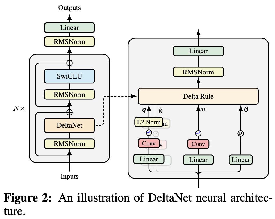Short Conv in DeltaNet

Why add this Short Conv? The intuitive explanation might be that it increases model depth, enhances the model's token-mixing ability, and so on — in other words, it compensates for the loss of expressive power caused by linearization. This explanation isn't wrong exactly, but it's a "one-size-fits-all" answer, and what we really want is a more precise understanding of the mechanism by which it works.

In what follows, I'll offer my own understanding (or, more accurately, my own guess). more

Train-Test

From A Brief History of Linear Attention: Imitation, Innovation, and Feedback we know that the core idea underlying today's new-style linear attention models is TTT (Test-Time Training), or in other words, online learning. TTT builds (not necessarily linear) RNN models by exploiting the similarity between optimizer updates and RNN iteration; linear attention variants such as DeltaNet, GDN, and Comba can all be viewed as special cases of it.

Specifically, TTT treats $\boldsymbol{K},\boldsymbol{V}$ as paired training data $(\boldsymbol{k}_1, \boldsymbol{v}_1),(\boldsymbol{k}_2, \boldsymbol{v}_2),\cdots,(\boldsymbol{k}_t, \boldsymbol{v}_t)$, which we use to train a model $\boldsymbol{v} = \boldsymbol{f}(\boldsymbol{S}_t;\boldsymbol{k})$, producing outputs $\boldsymbol{o}_t = \boldsymbol{f}(\boldsymbol{S}_t;\boldsymbol{q}_t)$, where $\boldsymbol{S}_t$ is the model parameter, updated via SGD:

\begin{equation} \boldsymbol{S}_t = \boldsymbol{S}_{t-1} - \eta_t\nabla_{\boldsymbol{S}_{t-1}}\mathcal{L}(\boldsymbol{f}(\boldsymbol{S}_{t-1};\boldsymbol{k}_t), \boldsymbol{v}_t)\end{equation}

Of course, if we like, we could also consider other optimizers — for instance Test-Time Training Done Right tries the Muon optimizer. Besides swapping out the optimizer, we're also free to change the architecture of the model $\boldsymbol{v} = \boldsymbol{f}(\boldsymbol{S}_t;\boldsymbol{k})$ and the loss function $\mathcal{L}(\boldsymbol{f}(\boldsymbol{S}_{t-1};\boldsymbol{k}_t), \boldsymbol{v}_t)$. Furthermore, we can also consider mini-batch TTT operating at the granularity of chunks.

It's not hard to imagine that, in principle, TTT is extremely flexible and can be used to construct arbitrarily complex RNN models. When the architecture is chosen to be a linear model $\boldsymbol{v} = \boldsymbol{S}_t\boldsymbol{k}$ and the loss function is chosen to be squared error, the result corresponds to DeltaNet; if we add some regularization terms on top of that, we can derive variants such as GDN.

A Probing Question

The reason for putting TTT front and center is to make clear that the underlying logic of current mainstream linear attention is the same as that of TTT: at its core, it is online learning over paired training data $(\boldsymbol{k}_1, \boldsymbol{v}_1),(\boldsymbol{k}_2, \boldsymbol{v}_2),\cdots,(\boldsymbol{k}_t, \boldsymbol{v}_t)$. This naturally raises a question: why do it this way? What exactly does this process learn?

To answer this, we first need to reflect on what it is we actually want. Given the characteristics of Softmax Attention, what we want is presumably to compute an $\boldsymbol{o}_t$ from $(\boldsymbol{k}_1, \boldsymbol{v}_1),(\boldsymbol{k}_2, \boldsymbol{v}_2),\cdots,(\boldsymbol{k}_t, \boldsymbol{v}_t)$ and $\boldsymbol{q}_t$, and ideally this process should depend on the entirety of $(\boldsymbol{k},\boldsymbol{v})$. At the same time, we want to achieve this with constant complexity, so an intuitive idea is to first compress $(\boldsymbol{k},\boldsymbol{v})$ into a fixed-size State (independent of $t$), and then read out from this State.

How do we achieve this compression? TTT's idea is: design a model $\boldsymbol{v} = \boldsymbol{f}(\boldsymbol{S}_t;\boldsymbol{k})$, and then use these $(\boldsymbol{k},\boldsymbol{v})$ pairs to "train" this model; once training is complete, the model has in some sense "memorized" these $(\boldsymbol{k},\boldsymbol{v})$ pairs, which amounts to compressing the entirety of $(\boldsymbol{k},\boldsymbol{v})$ into the fixed-size model weights $\boldsymbol{S}_t$. As for how $怎么利用$ makes use of $，直接将它代入模型中得到$, choosing $\boldsymbol{o}

_t = \boldsymbol{f}(\boldsymbol{S}_t;\boldsymbol{q}_t)$ is a fairly natural option, though in principle we could also devise other ways of making use of it.

That is to say, TTT's core task is to exploit the fact that "training a model" is approximately equivalent to "memorizing the training set," in order to achieve the compression of $\boldsymbol{K},\boldsymbol{V}$. However, the claim that "training a model" is approximately equivalent to "memorizing the training set" is not at all trivial — it comes with certain preconditions.

Same-Source Keys and Values

Here's an example: if we take $\boldsymbol{K}=\boldsymbol{V}$, then this TTT framework theoretically breaks down, because in that case the optimal solution for the model $\boldsymbol{v} = \boldsymbol{f}(\boldsymbol{S}_t;\boldsymbol{k})$ is simply the identity transformation — a trivial solution, equivalent to having memorized nothing at all. Online-update methods like DeltaNet might still salvage something, but exact-solution-based methods like MesaNet would genuinely just output the identity matrix $\boldsymbol{I}$.

Some readers might object: why on earth would we consider such an unreasonable choice as $\boldsymbol{K}=\boldsymbol{V}$ in the first place? Indeed, $\boldsymbol{K}=\boldsymbol{V}$ is a fairly extreme choice — it's used here only as an example, to illustrate that "training a model" being approximately equivalent to "memorizing the training set" doesn't hold unconditionally. Second, as we verified in The Path to the Upgraded Transformer: 20. What Makes MLA So Good? (Part 1), for Softmax Attention, $\boldsymbol{K}=\boldsymbol{V}$ can also achieve pretty good results.

This tells us that $\boldsymbol{K}=\boldsymbol{V}$ is not, in itself, a fundamental obstacle for the attention mechanism — but within the TTT framework it can cause the model to fail, precisely because when $\boldsymbol{K},\boldsymbol{V}$ fully coincide, there's nothing left for the regression between them to learn. Similarly, we can imagine that the higher the degree of information overlap between $\boldsymbol{K},\boldsymbol{V}$, the less there is to learn between them — in other words, the lower the degree to which TTT actually "memorizes" the training data.

In typical attention mechanisms, $\boldsymbol{q}_t,\boldsymbol{k}_t,\boldsymbol{v}_t$ are all obtained from the same input $\boldsymbol{x}_t$ via different linear projections — in other words, $\boldsymbol{k}_t,\boldsymbol{v}_t$ share the same source $\boldsymbol{x}_t$ — which always gives a certain feeling of "predicting itself from itself," leaving limited room for genuine learning.

Convolution to the Rescue

How can we get TTT to learn something more valuable even when keys and values share the same source, or even coincide ($\boldsymbol{K}=\boldsymbol{V}$)? Actually, the answer has been around for a long time — it can be traced back to Word2Vec, or even earlier — and it is: don't "predict yourself," predict what's around you instead.

Take Word2Vec as an example: we know it's trained via "the center word predicts the context"; the previously popular BERT used MLM as its pretraining task, where certain words are masked and then predicted — this can be described as "the context predicts the center word"; and mainstream LLMs today are trained on NTP (Next Token Prediction), predicting the next word given the preceding text. Clearly, what all of these have in common is that none of them predict themselves — they all predict what's nearby.

So, if we want to improve TTT, we need to change the "self-predicting-self" pairing scheme represented by $(\boldsymbol{k}_t,\boldsymbol{v}_t)$. Given that current LLMs are dominated by NTP, we can likewise consider NTP within TTT — for instance, using $(\boldsymbol{k}_{t-1},\boldsymbol{v}_t)$ to construct the training pairs, i.e., using $\boldsymbol{k}_{t-1}$ to predict $\boldsymbol{v}_t$. This way, even when $\boldsymbol{K}=\boldsymbol{V}$, we can still learn a non-trivial result. In this scheme, both the inner and outer tasks of TTT are NTP, giving a pleasing consistency.

However, using only $\boldsymbol{k}_{t-1}$ to predict $\boldsymbol{v}_t$ seems to waste $\boldsymbol{k}_t$, so a further idea is to mix $\boldsymbol{k}_{t-1}$ and $\boldsymbol{k}_t$ together in some way before predicting $\boldsymbol{v}_t$. At this point, you may already see where this is going: "mixing $\boldsymbol{k}_{t-1}$ and $\boldsymbol{k}_t$ together in some way" — isn't that exactly a convolution with kernel_size=2! So, adding Short Conv to $\boldsymbol{K}$ transforms TTT's training objective from "predict yourself" into NTP, giving TTT at least the capacity to learn an n-gram model.

As for adding Short Conv to $\boldsymbol{Q},\boldsymbol{V}$, that's essentially incidental. According to word from the FLA (Flash Linear Attention) group, adding it to $\boldsymbol{Q},\boldsymbol{V}$ does have some effect, but it's far less than the improvement brought by adding Short Conv to $\boldsymbol{K}$ — which lends some support to our conjecture.

Summary

This post offers a somewhat armchair-theorizing take on the question of why linear attention needs Short Conv.