MoE Time Travel: 5. Rethinking the Uniform Distribution

MoE环游记：5、均匀分布的反思 苏剑林 · 2025-05-16 · Machine Learning optimization sparse MoE

If Meta's LLAMA series established the standard architecture for Dense models, then DeepSeek is arguably the founder of the standard architecture for MoE. Of course, this doesn't mean DeepSeek invented MoE, nor that its MoE design is beyond improvement — rather, it means that several of the improvements DeepSeek has proposed for MoE are likely directions with quite significant effect gains, and are gradually becoming standard components of MoE. These include the Loss-Free load balancing scheme we introduced in MoE Time Travel: 3. A Different Way to Allocate, as well as the Shared Expert and Fine-Grained Expert strategies that this article will introduce.

Speaking of load balancing, it is undoubtedly one of the most important goals in MoE — the second through fourth articles in this series can be said to revolve entirely around it. However, some readers have gradually come to realize that there is an essential question here that remains unanswered: Setting aside efficiency considerations, is a uniform distribution necessarily the direction that gives the best performance? This article takes up this question as it explores Shared Expert and Fine-Grained Expert.

Shared Expert

Let's revisit the basic form of MoE once more:

\begin{equation}\boldsymbol{y} = \sum_{i\in \mathop{\text{argtop}}_k \boldsymbol{\rho}} \rho_i \boldsymbol{e}_i\end{equation}more

Beyond this, in MoE Time Travel: 3. A Different Way to Allocate the Loss-Free approach replaces $\mathop{\text{argtop}}_k \boldsymbol{\rho}$ with $\mathop{\text{argtop}}_k \boldsymbol{\rho}+\boldsymbol{b}$, and in MoE Time Travel: 4. Put More Effort Where It's Hard we generalized it to $\mathop{\text{argwhere}} \boldsymbol{\rho}+\boldsymbol{b} > 0$, but these variants are orthogonal to the Shared Expert technique, so in what follows we'll only use the most basic form as our example.

Shared Expert modifies the above formula to:

\begin{equation}\boldsymbol{y} = \sum_{i=1}^s \boldsymbol{e}_i + \sum_{i\in \mathop{\text{argtop}}_{k-s} \boldsymbol{\rho}_{[s:]}} \rho_{i+s} \boldsymbol{e}_{i+s}\label{eq:share-1}\end{equation}

That is, instead of selecting $k$ out of $n$, we now select $k-s$ out of $n-s$, with an additional $s$ Experts that are always selected regardless — these are called "Shared Experts" (when this first came out, we jokingly called them the "permanent members of the Security Council"), while the remaining $n-s$ Experts are called "Routed Experts." The number of Shared Experts, $s$, is usually not too large — typically 1 or 2 — since too many would end up "neglecting" the remaining Routed Experts.

It's worth pointing out that whether or not Shared Expert is enabled, the total number of Experts remains $n$, and the number of activated Experts remains $k$, so in principle Shared Expert does not increase the model's parameter count or inference cost. Even so, DeepSeekMoE and some of our own experiments show that Shared Expert can still improve model performance to some extent.

Multiple Perspectives

We can understand Shared Expert from several perspectives. Take the residual perspective: it suggests that the Shared Expert technique effectively changes the learning target for each Expert from learning the Expert itself to learning its residual relative to the Shared Expert, which lowers the learning difficulty and yields better gradients. In DeepSeek's own words: by compressing common knowledge into these Shared Experts, redundancy among Routed Experts is reduced, parameter efficiency is improved, and each Routed Expert is free to focus on its unique aspects.

If we compare Routed Experts to subject teachers in a middle school, then the Shared Expert is akin to the "homeroom teacher." If a class only had subject teachers, each of them would inevitably have to shoulder some administrative work; but by introducing the homeroom-teacher role, this shared administrative burden is concentrated on one teacher, freeing the subject teachers to focus on teaching and thereby improving teaching efficiency.

This can also be understood geometrically. The inevitable commonality among Experts corresponds geometrically to the angle between their vectors being less than 90 degrees, which contradicts the "pairwise orthogonality" assumption on Expert vectors that we used when introducing the geometric meaning of MoE in MoE Time Travel: 1. Starting From Geometric Meaning. While this assumption not holding exactly can still be treated as an approximate solution, naturally the closer it holds the better — and we can understand the Shared Expert as approximating the mean of these Routed Experts, so that by learning the residual after subtracting this mean, the orthogonality assumption becomes easier to satisfy.

Scaling Factor

Let's write the earlier formula $\eqref{eq:share-1}$ in a more general form:

\begin{equation}\boldsymbol{y} = \sum_{i=1}^s \boldsymbol{e}_i + \lambda\sum_{i\in \mathop{\text{argtop}}_{k-s} \boldsymbol{\rho}_{[s:]}} \rho_{i+s} \boldsymbol{e}_{i+s}\end{equation}

Since Routed Experts carry a weight $\rho_{i+s}$ while the Shared Expert doesn't, and since the number of Routed Experts is typically much larger than the number of Shared Experts (i.e., $n - s \gg s$), the balance between the two can easily become skewed. So, to keep neither side from being overwhelmed by the other, setting a reasonable $\lambda$ is particularly important. On this point, we proposed in Muon is Scalable for LLM Training that an appropriate $\lambda$ should make the norms of both sides roughly equal at initialization.

Specifically, we assume each Expert has the same norm at initialization (without loss of generality, this can be set to 1), and that the Experts are pairwise orthogonal. We further assume the Router's logits follow a standard normal distribution (i.e., zero mean, unit variance — though other variances could be considered if deemed necessary). Under these assumptions, the total norm of the $s$ Shared Experts is $\sqrt{s}$, while the total norm of the Routed Experts is

\begin{equation}\lambda\sqrt{\sum_{i\in \mathop{\text{argtop}}_{k-s} \boldsymbol{\rho}_{[s:]}} \rho_{i+s}^2}\end{equation}

By setting this equal to $\sqrt{s}$, we can estimate $\lambda$. Because the choice of activation function and whether or not renormalization is applied can cause considerable differences between different MoE Routers, rather than trying to find an analytical solution we simply run a numerical simulation:

import numpy as np

def sigmoid(x):
    return 1 / (1 + np.exp(-x))

def softmax(x):
    return (p := np.exp(x)) / p.sum()

def scaling_factor(n, k, s, act='softmax', renorm=False):
    factors = []
    for _ in range(10000):
        logits = np.random.randn(n - s)
        p = np.sort(eval(act)(logits))[::-1][:k - s]
        if renorm:
            p /= p.sum()
        factors.append(s**0.5 / (p**2).sum()**0.5)
    return np.mean(factors)

scaling_factor(162, 8, 2, 'softmax', False)
scaling_factor(257, 9, 1, 'sigmoid', True)

Remarkably, the simulation results from this script align very well with the settings used in DeepSeek-V2 and DeepSeek-V3. Specifically, DeepSeek-V2 has $n=162,k=8,s=2$, uses Softmax activation without renormalization, and the script's simulated result comes out to roughly 16 — which matches DeepSeek-V2's actual $\lambda$ of exactly 16 source ]. DeepSeek-V3, on the other hand, has $n=257,k=9,s=1$, uses Sigmoid activation with renormalization, and the script's result is about 2.83, while DeepSeek-V3's actual $\lambda$ is 2.5 source ].

Non-Uniformity

Let's return to the question posed at the start of this article: is balance necessarily the direction that yields the best performance? Shared Expert seems to offer a hint: not necessarily. Because Shared Expert can also be understood as certain Experts being always activated, meaning that, taken as a whole, this leads to a non-uniform distribution over Experts:

\begin{equation}\boldsymbol{F} = \frac{1}{s+1}\bigg[\underbrace{1,\cdots,1\\}_{s个},\underbrace{\frac{1}{n-s},\cdots,\frac{1}{n-s}\\}_{n-s 个}\bigg]\end{equation}

In fact, non-uniform distributions are everywhere in the real world, so it should be easy to accept that a uniform distribution isn't necessarily optimal. Let's return to our middle-school-teacher analogy: within any given school, the number of teachers per subject is in fact non-uniform — typically there are the most teachers for Chinese, Math, and English, fewer for Physics, Chemistry, and Biology, and even fewer for PE and Art (who also seem to call in sick more often). For more examples of non-uniform distributions, you might look up Zipf's law.

In short, the non-uniformity of the real world inevitably leads to non-uniformity in natural language, which in turn means that a uniform distribution is not optimal. Of course, from the standpoint of training a model, a uniform distribution is still much easier to parallelize and scale — so splitting off a small portion as Shared Experts, while still wanting the remaining Routed Experts to be uniform, is a compromise that achieves non-uniformity in a way that's friendly to both sides, rather than forcing the Routed Experts to directly conform to some non-uniform distribution.

That was about training — what about inference? During inference, we can estimate the actual distribution of Routed Experts in advance, and we don't need to worry about backpropagation, so with careful enough optimization it should in principle be possible to achieve this non-uniformity without any loss of efficiency. But because current MoE inference infrastructure is designed around a uniform distribution, and given practical constraints such as limited per-GPU memory, we still generally want the Routed Experts to be uniform in order to achieve better inference efficiency.

Finer Granularity

Besides Shared Expert, another improvement proposed by DeepSeekMoE is Fine-Grained Expert, which points out that, holding both the total parameter count and the activated parameter count fixed, finer Expert granularity tends to yield better performance.

For example, suppose we originally select $k$ out of $n$ Routed Experts; now if we shrink each Expert by half and instead select $2k$ out of $2n$, the total parameter count and the activated parameter count both stay the same, but the latter setup tends to perform better. The original paper's explanation is that this enriches the diversity of Expert combinations, i.e.,

\begin{equation}\binom{n}{k} \ll \binom{2n}{2k} \ll \binom{4n}{4k} \ll \cdots\end{equation}

Of course, there are other possible explanations too — for instance, further splitting an Expert into smaller units allows each Expert to focus on a narrower domain of knowledge, achieving a finer-grained decomposition of knowledge, and so on. But it's worth noting that Fine-Grained Expert is not free: the larger $n$ is, the more imbalanced the load among Experts tends to become, and the communication and coordination overhead between Experts also increases — so $n$ cannot be increased indefinitely either; there's a comfortable range that balances both effectiveness and efficiency.

Regarding why Fine-Grained Expert works, I'd like to offer another, less obvious explanation, one that connects back to the theme of this article: a larger number of finer-grained Experts can better approximate the non-uniformity of the real world. Take the figure below as an example: suppose knowledge can be divided into two categories, one large and one small, and each Expert is represented by a circle. If we try to cover this with 2 large circles, there will inevitably be some gaps and waste; but if we instead use 8 small circles of the same total area, the coverage becomes much finer and more precise, leading to better performance.

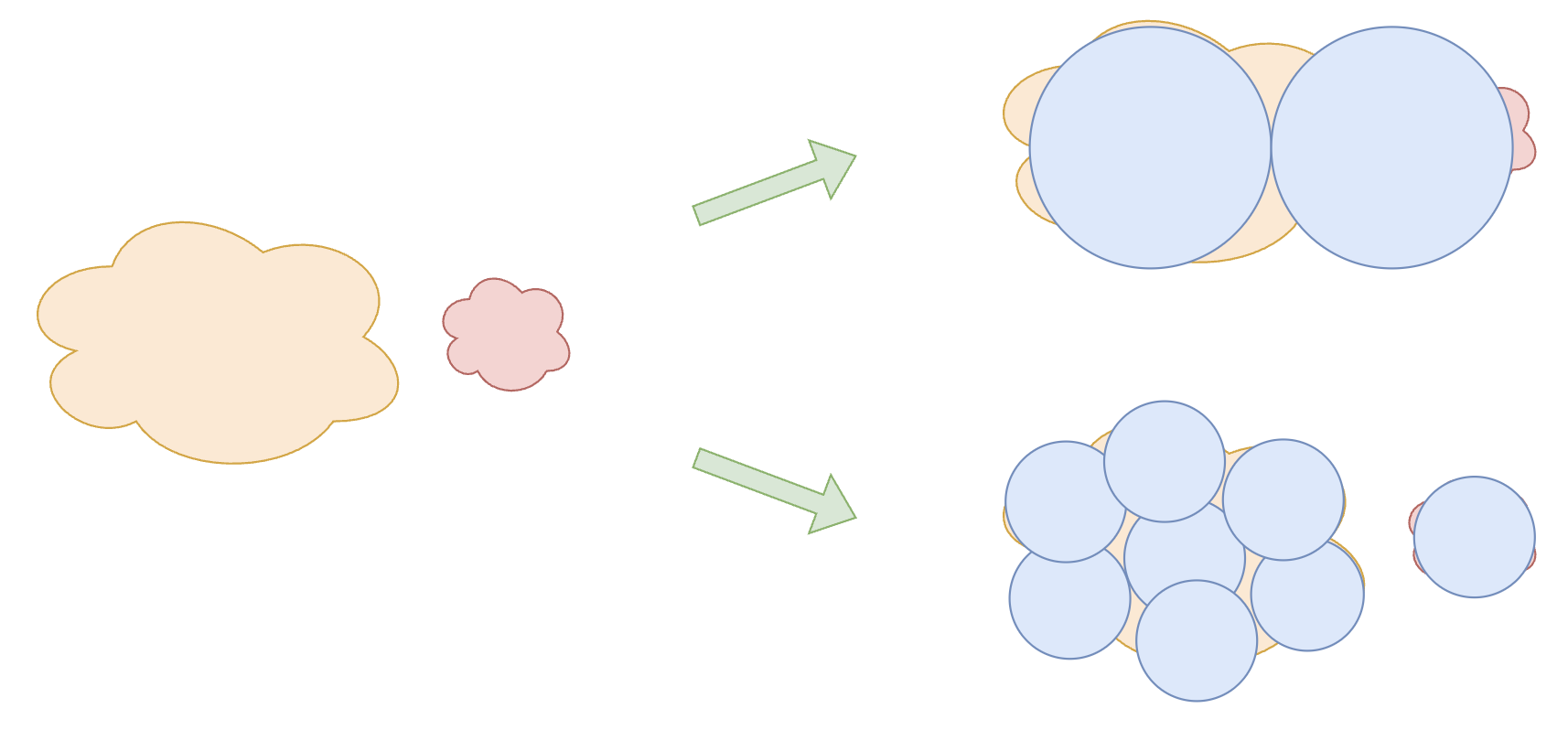Fine-grained coverage is more precise

Summary

This article introduced the Shared Expert and Fine-Grained Expert strategies for MoE, and pointed out that, to some extent, both of them reflect the sub-optimality of load balancing.