Monarch Matrices: A Computationally Efficient Sparse-Style Matrix Factorization
When it comes to matrix compression, we generally have two strategies to choose from: low-rank approximation and sparsification. Low-rank approximation reduces the size of a matrix by finding a low-rank approximation to it, while sparsification reduces the complexity of a matrix by cutting down its number of nonzero elements. If SVD is the go-to method for finding low-rank approximations of a matrix, then what algorithm plays the corresponding role for finding sparse approximations?
What we're going to look at next is the paper Monarch: Expressive Structured Matrices for Efficient and Accurate Training, which gives an answer to the question above — the "Monarch matrix." This is a family of matrices that can be decomposed into products of permutation matrices and sparse matrices, while at the same time being both computationally efficient and expressive. The paper also discusses how to find Monarch approximations of general matrices, as well as how to use Monarch matrices to parameterize LLMs in order to speed them up, among other things.
It's worth pointing out that the author of this paper is none other than Tri Dao, the famous author of Flash Attention, whose work almost entirely revolves around improving LLM performance. This Monarch paper is also one of the handful specially featured on his homepage, which alone makes it well worth studying. more
Recap of SVD
First let's briefly recap SVD (Singular Value Decomposition). For a matrix $A$ of size $n\times m$, SVD decomposes it as
\begin{equation}A = U\Sigma V\end{equation}
where $U,V$ are orthogonal matrices of shape $n\times n$ and $m\times m$ respectively, and $\Sigma$ is a $n\times m$ diagonal matrix whose diagonal entries are non-negative and arranged in decreasing order. When we keep only the first $r$ diagonal entries of $\Sigma$, we obtain a rank-at-most-$r$ approximate decomposition of $A$:
\begin{equation}A \approx U_{[:,:r]}\Sigma_{[:r,:r]} V_{[:r,:]}\end{equation}
Here the subscripts follow Python-style slicing, so $U_{[:,:r]}$ has shape $n\times r$, $\Sigma_{[:r,:r]}$ has shape $r\times r$, and $V_{[:r,:]}$ has shape $r\times m$, which means the rank of $U_{[:,:r]}\Sigma_{[:r,:r]} V_{[:r,:]}$ is at most $r$.
In particular, the low-rank approximation obtained via SVD above is exactly the precise solution to the following optimization problem:
\begin{equation}U_{[:,:r]}\Sigma_{[:r,:r]} V_{[:r,:]} = \mathop{\text{argmin}}_{rank(B)\leq r} \Vert A - B\Vert_F^2\end{equation}
where $\Vert\cdot\Vert_F^2$ is the square of the matrix's Frobenius norm, i.e., the sum of squares of every element of the matrix. In other words, under the Frobenius norm, the optimal rank-$r$ approximation to matrix $A$ is exactly $U_{[:,:r]}\Sigma_{[:r,:r]} V_{[:r,:]}$ — this result is known as the "Eckart–Young–Mirsky theorem." It is precisely because of this result that we said at the beginning of the article that "SVD is the go-to method for low-rank approximation of matrices."
There's a huge amount that could be said about SVD — enough to fill a whole book — so we won't go any deeper here. Finally, let's note that the computational complexity of SVD is $\mathcal{O}(nm\cdot\min(m,n))$, since we need to perform eigenvalue decomposition on at least one of $A^{\top} A$ or $A A^{\top}$. If we already know we're doing SVD in order to find a rank-$r$ approximation, the complexity can be reduced somewhat — this is Truncated SVD.
Monarch Matrices
Low-rank decomposition has extremely broad applications, but it doesn't necessarily always fit our needs. For instance, a low-rank approximation of an invertible square matrix is necessarily non-invertible, which means low-rank approximation isn't suitable for scenarios that require matrix inversion. In that case, another option is sparse approximation — sparse matrices can generally guarantee that the rank doesn't degenerate.
Note that sparsity and low rank have no necessary connection — for example, the identity matrix is very sparse, yet it is invertible (full rank). Finding a sparse approximation of a matrix isn't hard in itself: for instance, zeroing out all elements except the $k$ largest-in-absolute-value ones is a very naive sparse approximation. The problem is that this is usually not practical, so the real difficulty lies in finding a practical sparse approximation. By "practical," we mean retaining enough expressiveness or approximation quality while also achieving a certain degree of sparsification, and moreover having that sparsification follow a structure that helps speed up matrix operations (such as multiplication and inversion).
Monarch matrices were designed precisely for this purpose. Suppose $n=m^2$ is a perfect square; then the Monarch matrices form a subset of all $n$-order matrices, which we denote $\mathcal{M}^{(n)}$, defined as the set of matrices of the following form:
\begin{equation}M = PLPR\end{equation}
where $P$ are $n\times n$ permutation matrices (orthogonal matrices), and $L,R$ are block-diagonal matrices. Let's introduce each of these in turn.
Permutation Matrices
The permutation matrix $P$ has the effect of permuting the vector $[x_1,x_2,\cdots,x_n]$ into a new vector
\begin{equation}[x_1, x_{1+m}, \cdots , x_{1+(m−1)m}, x_2, x_{2+m}, \cdots , x_{2+(m−1)m}, \cdots , x_m, x_{2m}, \cdots , x_n]\end{equation}
Of course, written this way it may still seem confusing, but implementing it in code is actually very simple:
Px = x.reshape(m, m).transpose().reshape(n)
as shown in the figure below:
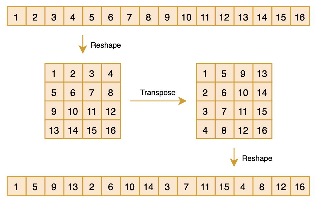 Illustration of the permutation matrix P
Readers who have worked on CV before might find this operation a bit familiar — it's essentially the "Shuffle" operation from ShuffleNet. This combined operation of first reshaping a vector, then transposing it, and finally reshaping it back, achieves a kind of "pseudo-shuffle" effect; it can also be viewed as a base-$m$ "bit-reversal permutation." Clearly, doing this operation twice restores the original vector, so we have $P^2=I$, and hence $P^{-1}=P^{\top}=P$.
Block-Diagonal Structure
Having discussed $P$, let's now talk about $L,R$. These are also matrices of size $n\times n$, but they are block-diagonal matrices of $m\times m$, with each block of size $m\times m$, as shown in the figure below:
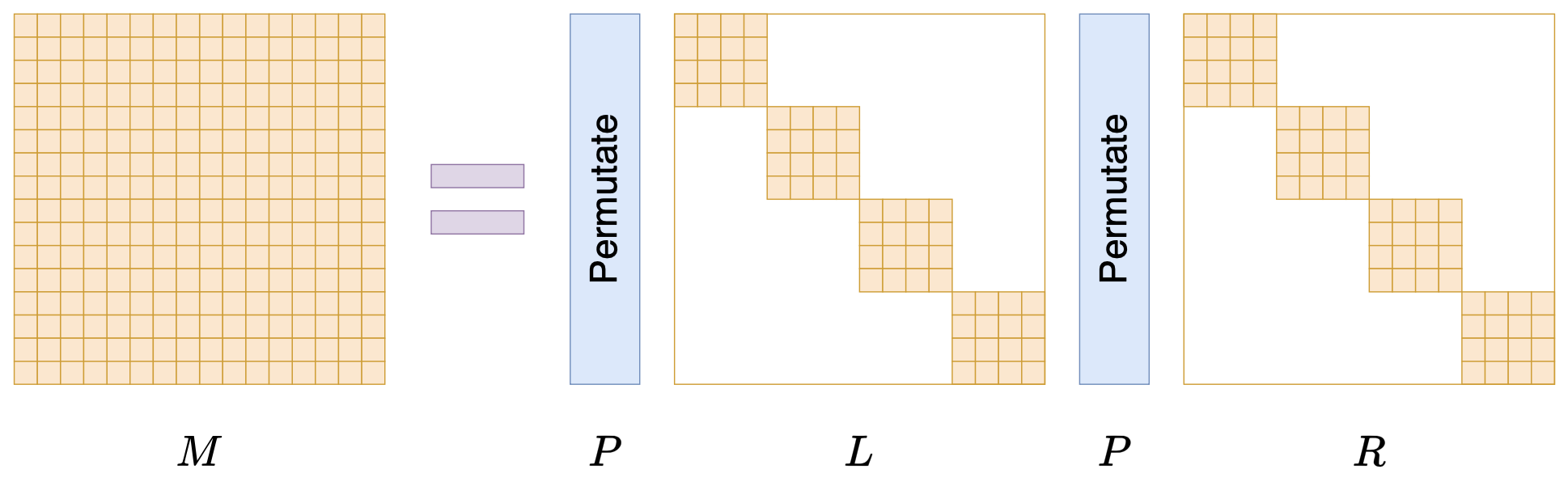 Monarch matrix form M=PLPR
When $n$ is sufficiently large, zeros dominate the count of entries in $L,R$, so $L,R$ are both sparse matrices — that is, the Monarch matrix is a matrix factorization form with sparse characteristics. Since $P$ is fixed, the variable elements in $PLPR$ all come from the nonzero elements of $L,R$. Therefore, although the matrix $M$ is a $n\times n$ matrix, its actual number of free parameters is no more than $2m^3=2n^{1.5}$. From this number $1.5$ we can already glimpse the intent behind Monarch matrices: they aim to take an operation that would normally require quadratic complexity and, via Monarch approximation, reduce it to complexity of order 1.5.
A Brief Efficiency Analysis
So can Monarch matrices actually achieve this goal? In other words, can Monarch matrices meet the "practical" standard mentioned earlier? We'll discuss expressiveness later; for now let's look at computational efficiency.
Take "matrix–vector" multiplication as an example. The standard complexity is $\mathcal{O}(n^2)$, but for a Monarch matrix we have $Mx = P(L(P(Rx)))$. Since multiplying by $P$ is just a simple reshape and transpose, it barely costs any computation at all — the main computational cost comes from multiplying $L$ or $R$ by a vector. Because of the block-diagonal nature of $L,R$, we can split the vector into $m$ groups, which turns the operation into $m$ separate multiplications of a $m\times m$ matrix by a $m$-dimensional vector, for a total complexity of $2m\times\mathcal{O}(m^2)=\mathcal{O}(2n^{1.5})$ — lower than $\mathcal{O}(n^2)$.
Another example is matrix inversion. Consider $M^{-1}x$: the standard complexity of inverting a $n$-order matrix is $\mathcal{O}(n^3)$, but for a Monarch matrix we have $M^{-1} x =R^{-1}PL^{-1}P x$. The main computational cost comes from $L^{-1}$, $R^{-1}$, and the corresponding "matrix–vector" multiplications. Since $L,R$ are both block-diagonal, we only need to invert each of the diagonal blocks separately — that is, a total of $2m$ inversions of $m\times m$ matrices, with complexity $2m\times\mathcal{O}(m^3)=\mathcal{O}(2n^2)$, again lower than the standard $\mathcal{O}(n^3)$. It's also possible to write $M^{-1}$ out explicitly, but doing so requires the identity $\eqref{eq:high-m-lr}$ introduced later.
So the conclusion is: because multiplication by $P$ costs essentially nothing, and because $L,R$ are block-diagonal matrices, operations related to a Monarch matrix of order $n$ can basically be reduced to independent operations on $2m$ matrices of size $m\times m$, thereby lowering the overall computational complexity. So at least on the front of computational efficiency, Monarch matrices hold up well. Moreover, since the nonzero elements of $L,R$ already have a square structure, they're also convenient to implement, allowing full use of the GPU without unnecessary waste.
Monarch Decomposition
Having confirmed the effectiveness of Monarch matrices, the next key question on the application side is: given an arbitrary $n=m^2$-order matrix $A$, how do we find its Monarch approximation? Similarly to SVD, we define the following optimization problem:
\begin{equation}\mathop{\text{argmin}}_{M\in\mathcal{M}^{(n)}} \Vert A - M\Vert_F^2\end{equation}
Fortunately, this problem admits a solution algorithm with complexity no greater than $\mathcal{O}(n^{2.5})$, which is even more efficient than SVD's $\mathcal{O}(n^3)$.
Higher-Dimensional Arrays
The key step to understanding this algorithm is converting the matrices and vectors related to Monarch matrices into higher-dimensional array form. Specifically, the Monarch matrix $M$ is originally a two-dimensional array, each of whose elements is denoted $M_{i,j}$, representing the element in row $i$ and column $j$. Now, following the block-matrix structure, we equivalently represent it as a four-dimensional array, whose elements we denote $M_{i,j,k,l}$, representing the element at big-row $i$, small-row $j$, big-column $k$, small-column $l$, as shown in the figure below:
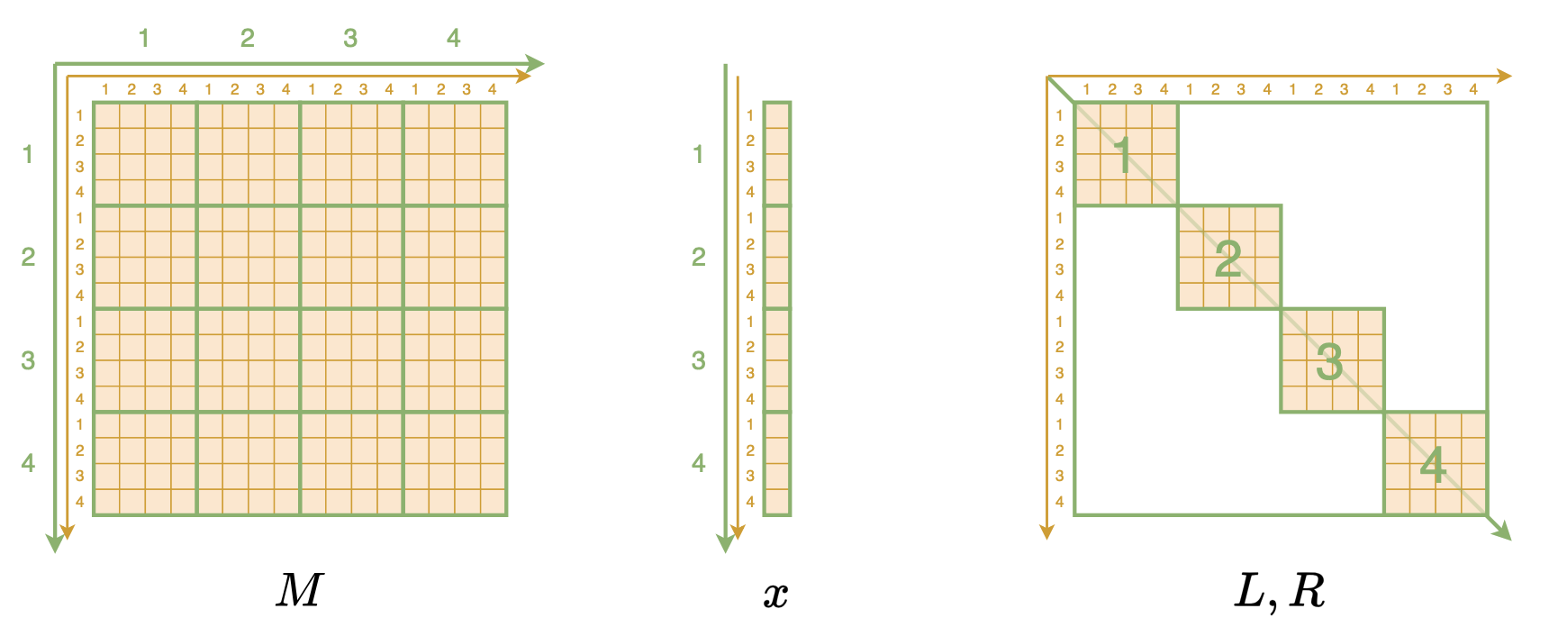 Viewing Monarch-related matrices/vectors as higher-dimensional arrays
Although this sounds like quite a mouthful, in code it's actually just one line:
M.reshape(m, m, m, m)
Similarly, the $n$-dimensional (column) vector $x$ is also converted into a two-dimensional array of shape $m\times m$, again in just one line of code x.reshape(m, m). As for the remaining $L,R$, it's naturally expressed as a three-dimensional array of shape $m\times m\times m$, where e.g. $L_{i,j,k}$ denotes the element at block $i$, small-row $j$, small-column $k$ — this is actually the most efficient way to store $L,R$, but for uniformity of treatment we can also lift it to four dimensions using the Kronecker delta symbol, e.g. $L_{i,j,k,l} = \delta_{i,k}L_{i,j,l}$, $R_{i,j,k,l} = \delta_{i,k}R_{i,j,l}$.
A New Identity
Next, we'll derive a new relation between $M$ and $L,R$. First, one can show that in the two-dimensional representation, multiplying the matrix $P$ by the vector $x$ becomes even simpler: the result is exactly the transpose of $x$, i.e. $(Px)_{i,j} = x_{j,i}$, and so we have $(PR)_{i,j,k,l} = R_{j,i,k,l} = \delta_{j,k}R_{j,i,l}$. Next, for the multiplication of two matrices, the four-dimensional representation has two summation indices, so
\begin{equation}(L P R)_{\alpha,\beta,k,l} = \sum_{i,j} L_{\alpha,\beta,i,j}(PR)_{i,j,k,l} = \sum_{i,j} \delta_{\alpha, i} L_{\alpha,\beta,j}\delta_{j,k}R_{j,i,l} = L_{\alpha,\beta,k}R_{k,\alpha,l}\end{equation}
Finally there's $(P L P R)_{\alpha,\beta,k,l}=L_{\beta,\alpha,k}R_{k,\beta,l}$: replacing $\alpha,\beta$ with $i,j$ gives $(P L P R)_{i,j,k,l}=L_{j,i,k}R_{k,j,l}$, and since $M=PLPR$, we have
\begin{equation}M_{i,j,k,l} = L_{j,i,k}R_{k,j,l}\label{eq:high-m-lr}\end{equation}
From this equation we can see that, when we fix a pair $(j,k)$, the left-hand side is a submatrix while the right-hand side is an outer product of two vectors. This means that if we want to find a Monarch approximation of a matrix $A$, we only need to convert $A$ into a four-dimensional array in the same way and, for each fixed pair $(j,k)$, the problem reduces to finding a "rank-1 approximation" of the corresponding submatrix! In other words, once we have this identity, finding a Monarch approximation of matrix $A$ can be reduced to finding rank-1 approximations for $m^2$ submatrices, which can be done using SVD, each with complexity no greater than $\mathcal{O}(m^3)$, so the total complexity is no greater than $m^2\times\mathcal{O}(m^3) = \mathcal{O}(n^{2.5})$.
Reference Implementation
Here's a simple reference implementation the author wrote in Numpy:
import numpy as np

def monarch_factorize(A):
    M = A.reshape(m, m, m, m).transpose(1, 2, 0, 3)
    U, S, V = np.linalg.svd(M)
    L = (U[:, :, :, 0] * S[:, :, :1]**0.5).transpose(0, 2, 1)
    R = (V[:, :, 0] * S[..., :1]**0.5).transpose(1, 0, 2)
    return L, R

def convert_3D_to_2D(LR):
    X = np.zeros((m, m, m, m))
    for i in range(m):
        X[i, i] += LR[i]
    return X.transpose(0, 2, 1, 3).reshape(n, n)

m = 8
n = m**2
A = np.where(np.random.rand(n, n) > 0.8, np.random.randn(n, n), 0)

L, R = monarch_factorize(A)
L = convert_3D_to_2D(L)
R = convert_3D_to_2D(R)
PL = L.reshape(m, m, n).transpose(1, 0, 2).reshape(n, n)
PR = R.reshape(m, m, n).transpose(1, 0, 2).reshape(n, n)

U, S, V = np.linalg.svd(A)

print('Monarch error:', np.square(A - PL.dot(PR)).mean())
print('Low-Rank error:', np.square(A - (U[:, :m] * S[:m]).dot(V[:m])).mean())
The author briefly compared this against the rank-$m$ approximation obtained via SVD (at which point the low-rank approximation and the Monarch approximation have a comparable number of parameters), and found that for fully dense matrices, the squared error of the rank-$m$ approximation tends to be (slightly) better than that of the Monarch approximation — which is expected, since it's clear from the Monarch approximation algorithm that it's essentially a customized version of SVD. However, if the matrix being approximated is a sparse matrix, then the Monarch approximation's error tends to be better, and the sparser it is, the more pronounced the advantage.
Generalizing Monarch
Up to this point, we've assumed that all the matrices under discussion are $n$-order square matrices, and that $n=m^2$ is a perfect square. While the square-matrix assumption may be acceptable, the requirement that $n=m^2$ be a perfect square is, after all, too restrictive. It's therefore worth at least generalizing the concept of the Monarch matrix to a non-square-number $n$.
Non-Square-Number Order
To do this, let's first introduce some notation. Suppose $b$ is a factor of $n$; let $\mathcal{BD}^{(b,n)}$ denote the set of all block-diagonal matrices of size $\frac{n}{b}\times \frac{n}{b}$ where each block is a submatrix of size $b\times b$ — clearly this generalizes the earlier $L,R$, and with this notation we can write $L,R\in\mathcal{BD}^{(\sqrt{n},n)}$. We also need to generalize the permutation matrix $P$: earlier we said the implementation of $P$ is Px = x.reshape(m, m).transpose().reshape(n), and now we generalize this to Px = x.reshape(n // b, b).transpose().reshape(n), denoted $P_{(\frac{n}{b},b)}$.
With this notation, we can define the general Monarch matrix (from the appendix of the original paper):
\begin{equation}\mathcal{M}^{(b,n)} = \Bigg\{M = P_{(b,\frac{n}{b})} L P_{(\frac{n}{b},b)} R\,\Bigg|\, L\in\mathcal{BD}^{(\frac{n}{b},n)}, R\in\mathcal{BD}^{(b,n)} \Bigg\}\end{equation}
Here's an illustration:
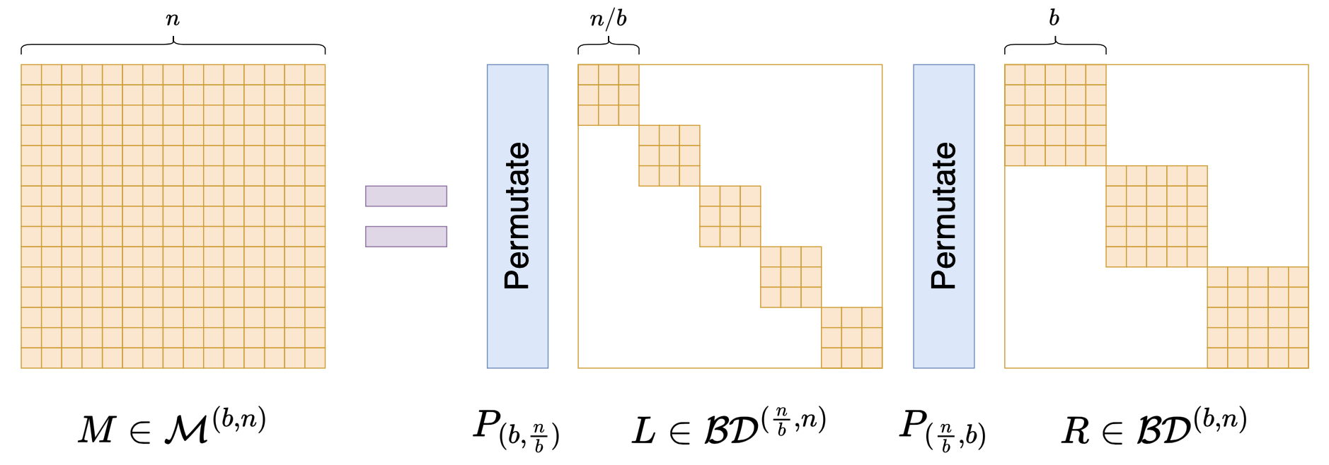 Generalizing the Monarch matrix to non-square-order square matrices
The Monarch matrix defined earlier can simply be denoted $\mathcal{M}^{(n)} = \mathcal{M}^{(\sqrt{n},n)}$ in this framework. It's not hard to compute that $L$ has at most $\frac{n^2}{b}$ nonzero elements, and $R$ has at most $nb$ nonzero elements, for a total of $\frac{n^2}{b} + nb$, which is minimized at $b=\sqrt{n}$ — so $b=\sqrt{n}$ is one of the sparsest cases.
Structure Is All That Matters
Readers might wonder: why distinguish between $L\in\mathcal{BD}^{(\frac{n}{b},n)}, R\in\mathcal{BD}^{(b,n)}$ at all — why not just use a single one? In fact, this design is precisely to ensure that the higher-dimensional identity $\eqref{eq:high-m-lr}$ still holds, so that a similar decomposition algorithm can be derived (we leave this as an exercise for the reader), and also to theoretically guarantee its expressiveness.
If we don't care about these theoretical details, and just want to construct a parameterization method with sparse characteristics, then we can generalize the Monarch matrix much more flexibly. For example:
\begin{equation}M = \left(\prod_{i=1}^k P_i B_i\right)P_0\end{equation}
where $B_1,B_2,\cdots,B_k \in \mathcal{BD}^{(b,n)}$, $P_0,P_1,\cdots,P_k$ are both permutation matrices, and the extra $P_0$ multiplied at the end is included purely for symmetry — it isn't strictly necessary. If you feel it's warranted, you could even choose a different $b$ for each $B_i$, i.e., $B_i\in \mathcal{BD}^{(b_i,n)}$.
You could even go further and combine this with low-rank decomposition, generalizing it to block matrices that aren't square, as shown below:
 Monarch-like matrix parameterization combining low rank and sparsity
Building on this analogy, we could further extend the concept of the Monarch matrix to non-square matrices. In short, if all you need is a sparsely-structured matrix similar in spirit to the Monarch matrix, without worrying about theoretical fine points, then the result is limited only by your imagination.
Application Examples
At present, the biggest selling point of Monarch matrices seems to be that they're friendly to matrix multiplication, so their most obvious use is simply replacing the parameter matrices of fully-connected layers to improve their efficiency — this is indeed the main focus of the experimental section of the original paper.
We can further divide this into "pre-processing" and "post-processing" approaches. "Pre-processing" means changing the parameter matrices of fully-connected layers to Monarch matrices before training the model, so that both training and inference are sped up, and the trained model best matches the Monarch matrix structure. "Post-processing" means we already have a trained model, and we use Monarch decomposition to find a Monarch approximation of the fully-connected layer's parameter matrix, then replace the original matrix with it, optionally fine-tuning briefly afterward — thereby improving the fine-tuning or inference efficiency of the original model.
Besides replacing fully-connected layers, Monarch Mixer: A Simple Sub-Quadratic GEMM-Based Architecture discusses an even more extreme approach — using it as a Token-Mixer module to directly replace the attention layer. However, in the author's view, Monarch-Mixer isn't especially elegant, because — like MLP-Mixer — it simply replaces the attention matrix with a learnable matrix, except here that matrix happens to be a Monarch matrix. This kind of design learns a static attention pattern, and one might reasonably question how well it generalizes.
Finally, for today's LLMs, Monarch matrices can also be used to build Parameter-Efficient Fine-Tuning (PEFT) schemes. As we know, LoRA was designed based on low-rank decomposition; and since low rank and sparsity are two parallel paths, shouldn't Monarch matrices — the flagship example of sparsity — also be usable for building a PEFT scheme? A quick search reveals that indeed someone has already done this: the paper is titled MoRe Fine-Tuning with 10x Fewer Parameters, quite fresh, from an ICML 2024 workshop.
Monarch of Butterflies
Let's finish with a brief discussion of the fitting capacity of Monarch matrices. "Monarch" means "emperor" or "sovereign," taken from the term "Monarch Butterfly." It's named this way because it's benchmarked against an earlier construct — the "Butterfly matrix."
What is a Butterfly matrix? This actually takes some explaining. A Butterfly matrix is a product of a series of ($\log_2 n$) Butterfly factor matrices, where each Butterfly factor matrix is itself a block-diagonal matrix whose diagonal blocks are called Butterfly factors (note: no "matrix" in the name). A Butterfly factor is in turn a $2\times 2$ block matrix, each of whose blocks is a diagonal matrix (and that's where the nesting ends). This is illustrated below:
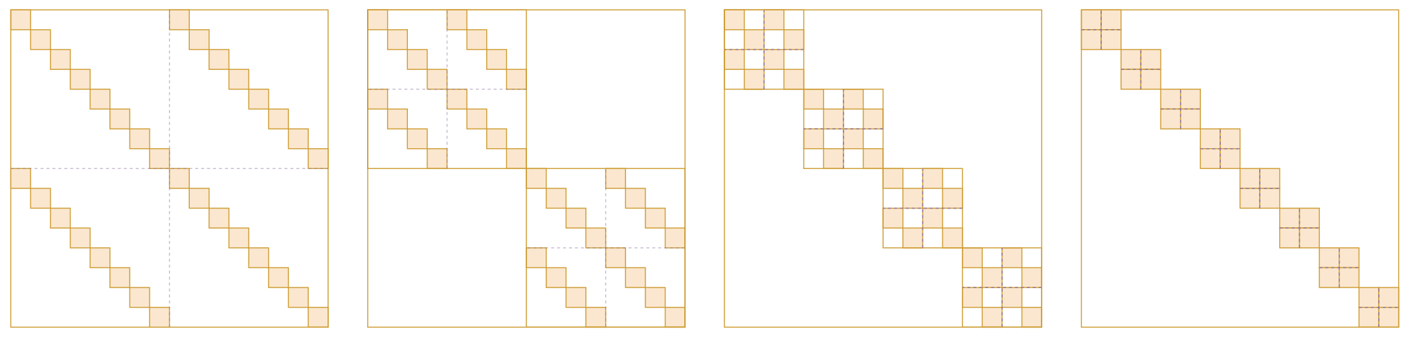 Illustration of the Butterfly matrix
For the precise definition of a Butterfly matrix, readers should consult the paper directly — we won't go into detail here. The name "Butterfly" comes from the author feeling that each Butterfly factor's shape resembles a butterfly; whether it actually does is up for debate, but the author clearly thought so. Literally speaking, "Monarch Butterfly" ranks above plain "Butterfly" (after all, it's the "emperor"), which hints that Monarch matrices are more powerful than Butterfly matrices. And indeed this is the case: the appendix of the Monarch paper proves that, no matter what value $b$ takes, $\mathcal{M}^{(b,n)}$ can cover all $n$-order Butterfly matrices, and when $n > 512$, $\mathcal{M}^{(b,n)}$ is strictly larger than the set of all $n$-order Butterfly matrices — in other words, anything a Butterfly matrix can do, a Monarch matrix can also do, but not necessarily vice versa.
We can also intuitively sense the expressive power of Monarch matrices from the complexity of "matrix–vector" multiplication. As we know, the standard complexity of multiplying an $n\times n$ matrix by a $n$-dimensional vector is $\mathcal{O}(n^2)$, but for certain structured matrices this can be lower — for example, the Fourier transform achieves $\mathcal{O}(n\log n)$, Butterfly matrices also achieve $\mathcal{O}(n\log n)$, and Monarch matrices achieve $\mathcal{O}(n^{1.5})$. So Monarch matrices "should" be no weaker than Butterfly matrices. Of course, Butterfly matrices also have their own advantages — for instance, their inverses and determinants are relatively easy to compute, which is more convenient for scenarios like Flow models that require computing inverses and determinants.
Summary
This article introduced the Monarch matrix, a family of matrices proposed by Tri Dao a couple of years ago that can be decomposed into a product of permutation matrices and sparse matrices, with the property of being computationally efficient (as everyone knows, Tri Dao is practically synonymous with high performance). Monarch matrices can be used to speed up fully-connected layers, to build parameter-efficient fine-tuning methods, and more.
Translated automatically with claude-sonnet-5; all equations are reproduced verbatim from the source. Copyright remains with the original author.