Revisiting SSM (Part 4): A New Perspective from Rational Generating Functions
In the previous three posts, we discussed most of the mathematical details of HiPPO and S4 in considerable depth. So what would you expect us to cover in this fourth installment? S5, Mamba, or even Mamba2? None of the above. This series is mainly concerned with the mathematical foundations of SSMs — the goal is to understand SSMs while also building up our own mathematical toolkit. We briefly mentioned S5 and Mamba in the previous post: S5 is a simplified version of S4 that introduces essentially no new mathematical techniques compared to S4, while the Mamba series, despite its excellent performance, has already simplified $A$ down to a diagonal matrix, so it uses even fewer new mathematical tricks — it's more a demonstration of engineering prowess.
In this post, we'll look at a new piece of work that hasn't yet received much attention, State-Free Inference of State-Space Models: The Transfer Function Approach (abbreviated RFT). It proposes a new scheme that moves the training, inference, and even parameterization of SSMs entirely into the space of generating functions, opening up a new perspective for understanding and applying SSMs.
Recap
Let's first briefly recap the results on S4 that we discussed in the previous post. S4 is based on the following linear RNN
\begin{equation}\begin{aligned} x_{k+1} =&\, \bar{A} x_k + \bar{B} u_k \\ y_{k+1} =&\, \bar{C}^* x_{k+1} \\ \end{aligned}\label{eq:linear}\end{equation}more
where $u,y\in\mathbb{R},x\in\mathbb{R}^d,\bar{A}\in\mathbb{R}^{d\times d},\bar{B},\bar{C}\in\mathbb{R}^{d\times 1}$. Here we want to keep the discussion general, so we'll bypass the relationship between $\bar{A}$ and $A$, and simply treat $\bar{A}$ as a general matrix. With a zero initial state, direct iteration gives us:
\begin{equation}y_L = \sum_{k=0}^L \bar{C}^*\bar{A}^k \bar{B}u_{L-k} = \bar{K}_{< L} * u_{< L} \end{equation}
where $*$ is a convolution operation, and
\begin{equation}\bar{K}_k = \bar{C}^*\bar{A}^k\bar{B},\quad \bar{K}_{< L} = \big(\bar{K}_0,\bar{K}_1,\cdots,\bar{K}_{L-1}\big),\quad u_{< L} = (u_0,u_1,\cdots,u_{L-1})\end{equation}
Since convolution can be computed efficiently via the discrete Fourier transform (DFT), the remaining problem is how to efficiently compute $\bar{K}$ — and this is the core contribution of S4. To this end, S4 introduces the generating function
\begin{align}\mathcal{G}(z|\bar{K}) =&\, \sum_{k=0}^{\infty} \bar{C}^*\bar{A}^k \bar{B}z^k = \bar{C}^*\left(I - z\bar{A}\right)^{-1}\bar{B} \\ \mathcal{G}_L(z|\bar{K}) =&\, \sum_{k=0}^{L-1} \bar{C}^*\bar{A}^k \bar{B}z^k = \bar{C}^*(I - z^L\bar{A}^L)\left(I - z\bar{A}\right)^{-1}\bar{B} \end{align}
If we can compute $\mathcal{G}_L(z|\bar{K})$ efficiently, we can substitute in $z=e^{-2i\pi l/L},l=0,1,2,\dots,L-1$ and the result is the DFT of $\bar{K}$, so after a further inverse transform (IDFT) we obtain $\bar{K}$. Since $z$ always satisfies $z^L=1$ at this point, we can also set $\tilde{C}^* = \bar{C}^*(I - \bar{A}^L)$, so that the form of $\mathcal{G}_L(z|\bar{K})$ matches $\mathcal{G}(z|\bar{K})$:
\begin{equation}\mathcal{G}_L(z|\bar{K}) = \tilde{C}^*\left(I - z\bar{A}\right)^{-1}\bar{B}\end{equation}
So how do we efficiently compute $\mathcal{G}(z|\bar{K})$ or $\mathcal{G}_L(z|\bar{K})$? S4 decomposes $\bar{A}$ into a "diagonal + low-rank" form and then computes it via the Woodbury identity, giving the final result
\begin{equation}\mathcal{G}(z|\bar{K}) = \frac{2}{1+z}\bar{C}^* \left[R_z^{-1} - R_z^{-1}u(I + v^*R_z^{-1}u)^{-1} v^*R_z^{-1}\right]B\end{equation}
where $R_z$ is a $d\times d$ diagonal matrix, and $u,v,B,\bar{C}$ are all column vectors of $d\times 1$. This means that given $z$, computing $\mathcal{G}(z|\bar{K})$ has complexity $\mathcal{O}(d)$, while computing over the full range of $z=e^{-2i\pi l/L},l=0,1,2,\dots,L-1$ naively costs $\mathcal{O}(Ld)$. S4 shows this can be reformulated as a Cauchy kernel problem, further reducing the complexity to $\mathcal{O}((L+d)\log^2(L+d))$.
Either way, we can see that the complexity depends not only on $L$ but also on $d$ (the state size). RFT instead proposes a new method that reduces the complexity directly to the ideal $\mathcal{O}(L\log L)$, independent of the state size — and the derivation is noticeably simpler than S4's, while also not depending on any assumption that $\bar{A}$ is diagonal or "diagonal + low-rank."
Rational Functions
RFT stands for Rational Transfer Function, and its focus is on rational functions, i.e., the ratio of two polynomials. What does this have to do with generating functions? The authors of RFT make the very clever observation that $\mathcal{G}_L(z|\bar{K})$ is in fact itself a rational function! Specifically, we have
\begin{equation}\mathcal{G}_L(z|\bar{K}) = \tilde{C}^*\left(I - z\bar{A}\right)^{-1}\bar{B} = \frac{b_1 + b_2 z + b_3 z^2 + \cdots + b_dz^{d-1}}{1 + a_1 z + a_2 z^2 + \cdots + a_d z^d}\label{eq:gz-rf}\end{equation}
where $a_1,a_2,\cdots,a_d,b_1,b_2,\cdots,b_d$ are all scalars — if $\bar{A},\bar{B},\tilde{C}$ are real matrices, these are all real numbers. If we just want to convince ourselves that such an equality exists, we only need to use a classical formula for matrix inversion:
\begin{equation}M^{-1} = \frac{\text{adj}(M)}{\det(M)}\end{equation}
where $\det(M)$ is the determinant of $M$, and $\text{adj}(M)$ is the adjugate matrix of $M$. Since the adjugate matrix involves a large number of determinant computations, this inversion formula is usually of little practical use for actual computation, but it often works wonders in theoretical analysis. For instance, substituting it into $\mathcal{G}_L(z|\bar{K})$ gives
\begin{equation}\mathcal{G}_L(z|\bar{K}) = \tilde{C}^*\left(I - z\bar{A}\right)^{-1}\bar{B} = \frac{\tilde{C}^*\text{adj}(I - z\bar{A})\bar{B}}{\det(I - z\bar{A})}\end{equation}
We know that a $d$-order determinant is a sum of products of $d$ elements, so $\det(I - z\bar{A})$ is a degree-$d$ polynomial in $z$. Next, by the definition of the adjugate matrix, each of its entries is a $d-1$-order determinant, i.e., a degree-$d-1$ polynomial; left-multiplying by $\tilde{C}^*$ and right-multiplying by $\bar{B}$ is just a weighted sum of these entries, so the result is still a degree-$d-1$ polynomial. Therefore, $\mathcal{G}_L(z|\bar{K})$ is a degree-$d-1$ determinant polynomial of $z$ divided by a degree-$d$ determinant polynomial of $z$; after normalizing the constant coefficient of the denominator to $1$, we obtain equation $\eqref{eq:gz-rf}$.
Correspondence
Furthermore, we can use a determinant identity to establish the relationship between the coefficients $a=(a_1,a_2,\cdots,a_d),b=(b_1,b_2,\cdots,b_d)$ and $\bar{A},\bar{B},\tilde{C}$. This identity is
\begin{equation}\det(I + UV) = \det(I + VU)\label{eq:det-iuv}\end{equation}
Proving this determinant identity directly isn't hard — it's the kind of thing you might see in a graduate entrance exam — you just need to note that
\begin{equation}\begin{pmatrix}I & U \\ -V & I\end{pmatrix} = \begin{pmatrix}I + UV & U \\ 0 & I\end{pmatrix}\begin{pmatrix}I & 0 \\ -V & I\end{pmatrix} = \begin{pmatrix}I & 0 \\ -V & I + VU\end{pmatrix}\begin{pmatrix}I & U \\ 0 & I\end{pmatrix}\end{equation}
By the definition and form of the determinant, the middle determinant is $\det(I + UV)$, and the rightmost determinant is $\det(I + VU)$; since these are determinants of the same matrix, the results must be equal. This result can be further generalized (when $A,D$ are invertible) to
\begin{equation}\det\begin{pmatrix}A & B \\ C & D\end{pmatrix} = \det(A)\det(D-CA^{-1}B) = \det(D)\det(A-BD^{-1}C)\end{equation}
Going even further, this can be generalized into the "Schur complement" theory that we mentioned in The KL Divergence, Bhattacharyya Distance, and Wasserstein Distance Between Two Multivariate Gaussians.
Back to the main thread: note that in deriving equation $\eqref{eq:det-iuv}$, we never needed to assume that $U,V$ are square matrices, so equation $\eqref{eq:det-iuv}$ actually holds even for non-square matrices, as long as the identity matrix $I$ automatically matches the sizes of $UV$ and $VU$. In particular, if $U,V$ are a column vector and a row vector respectively, then $VU$ is a scalar, the corresponding $I$ is 1, and its determinant is just itself, i.e., $\det(I + UV) = 1 + VU$. Using this special case, we get
\begin{equation}\begin{aligned} \mathcal{G}_L(z|\bar{K}) =&\, z^{-1}\left[1+\tilde{C}^*\left(z^{-1}I - \bar{A}\right)^{-1}\bar{B} - 1 \right]\\ =&\, z^{-1}\left[\det\left(I + \left(z^{-1} I - \bar{A}\right)^{-1}\bar{B}\tilde{C}^*\right) - 1\right]\\ =&\, z^{-1}\left\{\det\left[\left(z^{-1} I - \bar{A}\right)^{-1}\left(z^{-1} I - \bar{A} + \bar{B}\tilde{C}^*\right)\right] - 1\right\} \\ =&\, z^{-1}\left[\frac{\det(z^{-1} I - \bar{A} + \bar{B}\tilde{C}^*)}{\det(z^{-1} I - \bar{A})} - 1\right] \\ =&\, \frac{z^{d-1}\left[\det(z^{-1} I - \bar{A} + \bar{B}\tilde{C}^*)-\det(z^{-1} I - \bar{A})\right]}{z^d\det(z^{-1} I - \bar{A})} \\ \end{aligned}\end{equation}
In the denominator, $\det(z^{-1} I - \bar{A})$ is the characteristic polynomial of the matrix $\bar{A}$ in the variable $\lambda=z^{-1}$ — a monic degree-$d$ polynomial in $z^{-1}$ — and multiplying by $z^d$ turns it into a degree-$d$ polynomial in $z$ with constant term 1. Similarly, in the numerator, $\det(z^{-1} I - \bar{A} + \bar{B}\tilde{C}^*)$ is the characteristic polynomial of $\bar{A} - \bar{B}\tilde{C}^*$ (a monic degree-$d$ polynomial in $z^{-1}$); subtracting $\det(z^{-1} I - \bar{A})$ leaves exactly a degree-$d-1$ polynomial in $z^{-1}$, and multiplying by $z^{d-1}$ turns it into a degree-$d-1$ polynomial in $z$. So the vector $a$ is precisely the coefficients of the polynomial $\det(\lambda I - \bar{A})$ excluding the leading term, and the vector $b$ is the coefficients of the polynomial $\det(\lambda I - \bar{A} + \bar{B}\tilde{C}^*)-\det(\lambda I - \bar{A})$ (ordered from highest to lowest degree).
A Pleasant Surprise
Let's pause here for a moment and think about what we've done and where we're headed.
Our starting point is the linear system $\eqref{eq:linear}$. To make it parallelizable for training, we recast it as a convolution between $\bar{K}_{< L}$ and $u_{< L}$, which can then be computed efficiently via DFT, pointwise multiplication, and IDFT — so efficiency isn't a problem at that step. Now $u_{< L}$ is readily available, but $\bar{K}_{< L}$ is unknown, so the problem becomes how to efficiently compute the convolution kernel $\bar{K}_{< L}=\{\tilde{C}^*\bar{A}^k\bar{B}\}_{k=0}^{L-1}$. To this end, we further introduced the generating function $\mathcal{G}_L(z|\bar{K})$: as long as we can compute $\mathcal{G}_L(z|\bar{K})$ efficiently, we have
\begin{equation}DFT(\bar{K}_{< L}) = \Big\{\mathcal{G}_L(z|\bar{K})\Big\}_{z=e^{-2i\pi l/L},l=0,1,2,\dots,L-1}\end{equation}
and then IDFT can recover the original $\bar{K}_{< L}$. For $z=e^{-2i\pi l/L}$, we have $z^L=1$, so
\begin{equation}\mathcal{G}_L(z|\bar{K}) = \tilde{C}^*(I - z^L\bar{A}^L)\left(I - z\bar{A}\right)^{-1}\bar{B} = \underbrace{\bar{C}^*(I - \bar{A}^L)}_{\tilde{C}^*}\left(I - z\bar{A}\right)^{-1}\bar{B} \end{equation}
That is, we can treat the entire $\bar{C}^*(I - \bar{A}^L)$ as trainable parameters $\tilde{C}^*$, and only afterward solve for the corresponding $\bar{C}$ to use for inference.
S4 computes $\mathcal{G}_L(z|\bar{K})$ via a "diagonal + low-rank" decomposition, whereas this new paper points out that $\mathcal{G}_L(z|\bar{K})$ is actually a rational function, i.e., equation $\eqref{eq:gz-rf}$. If we substitute $z=e^{-2i\pi l/L}$ at this point, we find some genuinely delightful results — for instance, the denominator
\begin{equation}1 + a_1 z + a_2 z^2 + \cdots + a_d z^d = \sum_{k=0}^L a_k z^k = \sum_{k=0}^L a_k e^{-2i\pi kl/L} = DFT(\bar{a}_{< L})\end{equation}
where $\bar{a}_{< L} = (a_0,a_1,a_2,\cdots,a_{L-1}) = (1, a_1,a_2, \cdots, a_d, 0, \cdots, 0)$ — that is, by definition, the denominator is exactly the DFT of $a$ prepended with a 1 and padded with zeros on the right, up to a total length of $L$! Likewise, defining $\bar{b}_{< L} = (b_1,b_2,\cdots,b_d,0,0,\cdots,0)$, the numerator becomes $DFT(\bar{b}_{< L})$, so we can simply write
\begin{equation}DFT(\bar{K}_{< L}) = \frac{DFT(\bar{b}_{< L})}{DFT(\bar{a}_{< L})} = \frac{DFT(b_1,b_2,\cdots,b_d,0,0,\cdots,0)}{DFT(1, a_1,a_2, \cdots, a_d, 0, \cdots, 0)}\end{equation}
and then IDFT gives us $\bar{K}_{< L}$, where both the DFT and IDFT have computational complexity $\mathcal{O}(L\log L)$, independent of $d$ (we only need $d < L$)! This is the core idea behind why RTF's complexity is independent of the state size $d$.
Starting from Scratch
Following the order of introduction above, our computational process would be: first given $\bar{A},\bar{B},\tilde{C}$, then compute the coefficients of the characteristic polynomials of $\bar{A}$ and $\bar{A}-\bar{B}\tilde{C}^*$, thereby obtaining $a_1,a_2, \cdots, a_d$ and $b_1,b_2,b_3,\cdots,b_d$, and finally compute the DFT, divide, and IDFT to obtain $\bar{K}_{< L}$. For pure computation this poses no issue, but we're dealing with a training scenario where $\bar{A},\bar{B},\tilde{C}$ may carry trainable parameters, and in that case computing the characteristic polynomials of $\bar{A}$ and $\bar{A}-\bar{B}\tilde{C}^*$ makes gradient propagation through this step rather awkward.
A cleaner solution to this problem is to "start from scratch" — take the RTF form of equation $\eqref{eq:gz-rf}$ directly as the starting point, and set $a=(a_1,a_2, \cdots, a_d)$ and $b=(b_1,b_2,b_3,\cdots,b_d)$ as the trainable parameters themselves. Then we skip the characteristic polynomial computation entirely and can directly compute $\bar{K}_{\leq L}$ via DFT and IDFT. Moreover, whereas $\bar{A},\bar{B},\tilde{C}$ originally had $d^2+2d$ parameters, the two vectors $a,b$ now have only $2d$ parameters in total, greatly reducing the parameter count. And since any $\bar{A},\bar{B},\tilde{C}$ can be mapped to a corresponding $a,b$, the theoretical expressive power of RFT is no less than that of the original RNN form.
Of course, RTF only provides a way to train efficiently by directly using $a,b$ as the parameters; if we want step-by-step inference, we still need to convert back to the RNN form. This means that, given a trained $a,b$, we need to find a set of values $\bar{A},\bar{B},\tilde{C}$ and then substitute them into equation $\eqref{eq:linear}$ for inference. Note that $a,b\to\bar{A},\bar{B},\tilde{C}$ is a mapping from $2d$ parameters to $d^2+2d$ parameters, so there are certainly infinitely many solutions — we just need to find one that's as simple as possible.
The Companion Matrix
How do we find such a solution? We already showed above that the vector $a$ is exactly the coefficients of the polynomial $\det(z I - \bar{A})$ excluding the leading term, so finding $\bar{A}$ given $a$ amounts to, given a characteristic polynomial, finding a corresponding matrix. The simplest solution is a diagonal matrix: let $\lambda_1,\lambda_2,\cdots,\lambda_d$ be the $d$ roots of $\lambda^d + a_1 \lambda^{d-1} + a_2 \lambda^{d-2} + \cdots + a_d =0$, and then just set $\bar{A}=\text{diag}(\lambda_1,\lambda_2,\cdots,\lambda_d)$. However, this may introduce complex roots, which is somewhat unsatisfying, and moreover this kind of purely formal solution doesn't let us directly observe the relationship between $\bar{A}$ and $a$.
In fact, the problem of finding a real matrix whose characteristic polynomial equals a given real polynomial has long been studied, and its answer has an interesting name: the "companion matrix," which takes the form (to match the results of the original paper, this has an extra flip compared to the Wikipedia convention):
\begin{equation}\bar{A} = \begin{pmatrix}-a_1 & - a_2 & \cdots & -a_{d-1} & -a_d \\ 1 & 0 & \cdots & 0 & 0 \\ 0 & 1 & \cdots & 0 & 0 \\ \vdots & \vdots & \ddots & \vdots & \vdots \\ 0 & 0 & \cdots & 1 & 0 \\ \end{pmatrix}\label{eq:bar-A}\end{equation}
Proving after the fact that this matrix satisfies
\begin{equation}\det(\lambda I-\bar{A})=\lambda^d + a_1 \lambda^{d-1} + a_2 \lambda^{d-2} + \cdots + a_d\end{equation}
isn't difficult — just expand the determinant of $\det(\lambda I-\bar{A})$ along its first row directly. The more profound question is how one might come up with this construction in the first place; here I'll offer my own take. Constructing a matrix from a characteristic polynomial is, at its core, about progressively transforming the polynomial into a determinant where $\lambda$ appears only on the diagonal. For instance, when $d=2$ we have
\begin{equation}\lambda^2 + a_1 \lambda + a_2 = (\lambda + a_1)\lambda - (-1) \times a_2 ) = \det\begin{pmatrix} \lambda + a_1 & a_2 \\ -1 & \lambda\end{pmatrix}\end{equation}
from which we can extract the corresponding $\bar{A}$. For general $d$, we have
\begin{equation}\lambda^d + a_1 \lambda^{d-1} + a_2 \lambda^{d-2} + \cdots + a_d = \det\begin{pmatrix} \lambda^{d-1} + a_1 \lambda^{d-2} + \cdots + a_{d-1} & a_d \\ -1 & \lambda\end{pmatrix}\end{equation}
This still isn't the final answer, of course, but it does successfully reduce the degree of the polynomial by one, which suggests that we might try building this recursively — putting a matrix constructed from the characteristic polynomial $\lambda^{d-1} + a_1 \lambda^{d-2} + \cdots + a_{d-1}$ in the top-left corner, then tweaking the top-right and bottom-left entries slightly to form a block matrix. With a bit of careful experimentation, one has a real chance of arriving at the result in equation $\eqref{eq:bar-A}$ oneself.
Once we have $\bar{A}$, constructing $\bar{B},\tilde{C}$ becomes much easier. Again, by our earlier conclusion, we have
\begin{equation}\begin{gathered} \det(\lambda I - \bar{A} + \bar{B}\tilde{C}^*)-\det(\lambda I - \bar{A}) = b_1 \lambda^{d-1} + b_2 \lambda^{d-2} + \cdots + b_d \\ \Downarrow \\ \det(\lambda I - \bar{A} + \bar{B}\tilde{C}^*)= \lambda^d + (a_1 + b_1) \lambda^{d-1} + (a_2+b_2) \lambda^{d-2} + \cdots + (a_d + b_d) \end{gathered}\end{equation}
meaning that the characteristic polynomial of $\bar{A} - \bar{B}\tilde{C}^*$ is the expression above; so by the construction of $\bar{A}$, we obtain one solution for $\bar{A} - \bar{B}\tilde{C}^*$:
\begin{equation}\bar{A} - \bar{B}\tilde{C}^* = \begin{pmatrix}-a_1 - b_1 & - a_2 - b_2 & \cdots & -a_{d-1} - b_{d-1} & -a_d - b_d\\ 1 & 0 & \cdots & 0 & 0 \\ 0 & 1 & \cdots & 0 & 0 \\ \vdots & \vdots & \ddots & \vdots & \vdots \\ 0 & 0 & \cdots & 1 & 0 \\ \end{pmatrix}\end{equation}
and hence
\begin{equation}\bar{B}\tilde{C}^* = \begin{pmatrix}b_1 & b_2 & \cdots & b_{d-1} & b_d\\ 0 & 0 & \cdots & 0 & 0 \\ 0 & 0 & \cdots & 0 & 0 \\ \vdots & \vdots & \ddots & \vdots & \vdots \\ 0 & 0 & \cdots & 0 & 0 \\ \end{pmatrix} = \begin{pmatrix}1 \\ 0 \\ \vdots \\ 0 \\ 0\end{pmatrix}\begin{pmatrix}b_1 & b_2 & \cdots & b_{d-1} & b_d\end{pmatrix}\end{equation}
This means we can find a set of solutions $\bar{B} = [1, 0, \cdots, 0, 0], \tilde{C}^* = [b_1 , b_2 , \cdots , b_{d-1} , b_d]$, and then further solve for $\bar{C}^* = \tilde{C}^*(I - \bar{A}^L)^{-1}$.
The Initialization Scheme
Let's write out the recursive form of $x_k$ in full:
\begin{equation} x_{k+1} = \begin{pmatrix}-a_1 & - a_2 & \cdots & -a_{d-1} & -a_d \\ 1 & 0 & \cdots & 0 & 0 \\ 0 & 1 & \cdots & 0 & 0 \\ \vdots & \vdots & \ddots & \vdots & \vdots \\ 0 & 0 & \cdots & 1 & 0 \\ \end{pmatrix} x_k + \begin{pmatrix}1 \\ 0 \\ \vdots \\ 0 \\ 0\end{pmatrix} u_k = \begin{pmatrix} u_k - \langle a, x_k\rangle \\ x_{k,(0)} \\ x_{k,(1)} \\ \vdots \\ x_{k,(d-3)} \\ x_{k,(d-2)}\end{pmatrix} \end{equation}
Thanks to the extreme sparsity of $\bar{A}$, each recursion step can be completed in $\mathcal{O}(d)$ rather than $\mathcal{O}(d^2)$. In particular, when $a_1=a_2=\cdots=a_d=0$, we get:
\begin{equation}\begin{aligned} x_1 =&\, [u_0,0,\cdots,0] \\ x_2 =&\, [u_1,u_0,0,\cdots,0] \\ &\vdots \\ x_d =&\, [u_{d-1},\cdots,u_1,u_0] \\ x_{d+1} =&\, [u_d, u_{d-1},\cdots,u_1] \\ &\vdots \\ \end{aligned}\end{equation}
That is, the model is continually rolling forward and storing the most recent $d$ values of $u_k$. In the absence of any other prior knowledge, this is clearly a very sensible starting solution, and indeed the original paper sets $a_1,a_2,\cdots,a_d$ to zero during initialization.
The original paper offers another interpretation of this initialization, one that enhances numerical stability and prevents gradient explosion. From the previous post, we know that the linear system $\eqref{eq:linear}$ is invariant under similarity transformations, meaning that its dynamics are mathematically identical to the dynamics obtained after diagonalizing $\bar{A}$. The diagonalizing matrix of $\bar{A}$ is the diagonal matrix formed from all the zeros of its characteristic polynomial; if any zero $\lambda_k$ has modulus greater than 1, then after many steps of recursion numerical/gradient explosion can occur.
In other words, we would ideally like to constrain $a_1,a_2,\cdots,a_d$ so that all the zeros of the polynomial $\lambda^d + a_1 \lambda^{d-1} + a_2 \lambda^{d-2} + \cdots + a_d$ have modulus no greater than 1, in order to achieve better numerical stability while avoiding gradient explosion. However, a necessary and sufficient condition guaranteeing that all zeros of a polynomial lie within the unit circle is still not known; but a relatively simple sufficient condition is $|a_1| + |a_2| + \cdots + |a_d| < 1$.
Claim: When $|a_1| + |a_2| + \cdots + |a_d| < 1$, all the zeros of the polynomial $\lambda^d + a_1 \lambda^{d-1} + a_2 \lambda^{d-2} + \cdots + a_d$ have modulus no greater than 1.
Proof: By contradiction. Suppose the polynomial has a zero $\lambda_0$ with modulus greater than 1, so $|\lambda_0^{-1}| < 1$. Then
\begin{equation}\begin{aligned} > 1 =&\, -a_1\lambda_0^{-1}-a_2\lambda_0^{-2}-\cdots-a_d \lambda_0^{-d} \\ > \leq &\, |a_1\lambda_0^{-1}+a_2\lambda_0^{-2}+\cdots+a_d \lambda_0^{-d}| \\ > \leq &\, |a_1\lambda_0^{-1}|+|a_2\lambda_0^{-2}|+\cdots+|a_d \lambda_0^{-d}| \\ > \leq &\, |a_1|+|a_2|+\cdots+|a_d| \\ > < &\, 1 > \end{aligned}\end{equation}
which produces the contradiction $1 < 1$. Hence the assumption is false, and all zeros of the polynomial have modulus no greater than 1.
However, RTF points out that directly constraining $a_1,a_2,\cdots,a_d$ to satisfy $|a_1| + |a_2| + \cdots + |a_d| < 1$ would substantially weaken the model's expressive power, doing more harm than good. RTF further finds that it suffices to satisfy this condition as closely as possible at initialization, and then let the model gradually learn on its own from there. The value that most fully satisfies this condition is naturally $a_1=a_2=\cdots=a_d=0$, which is why RTF adopts all-zero initialization.
Experimental Results
For the experimental section, the following two figures illustrate RTF's key characteristics:
 RTF's complexity is essentially independent of state size
 RTF can improve performance by increasing the state size
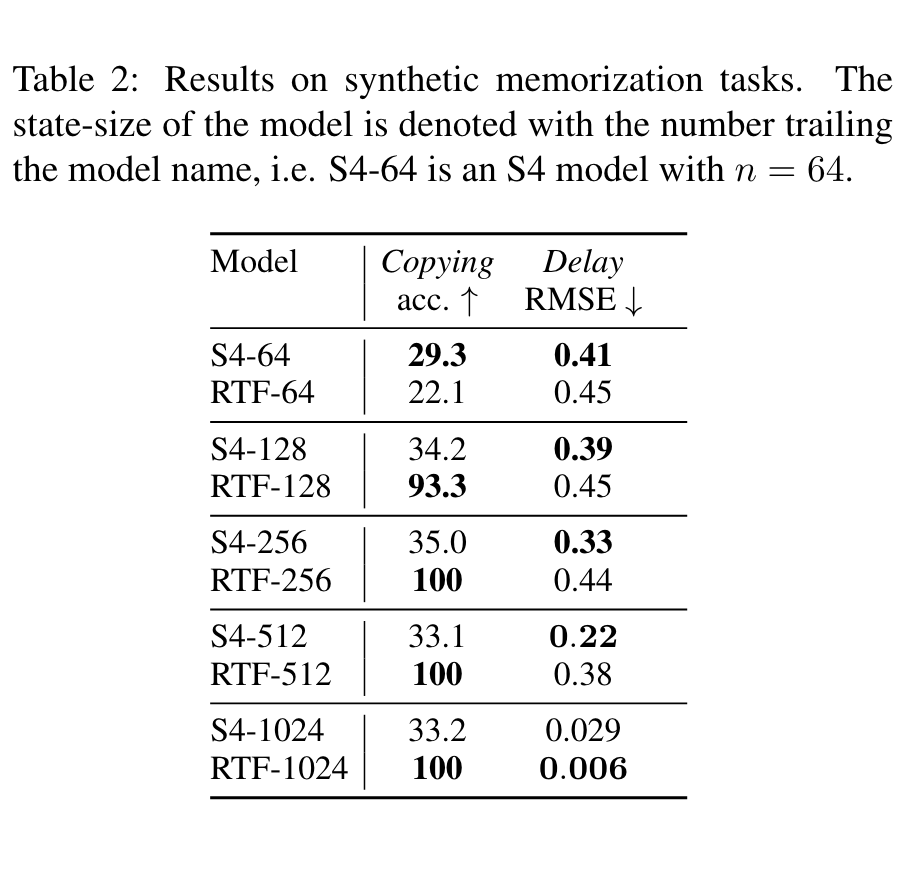
The first figure shows that RTF's computational complexity (both time and space) has no noticeable dependence on the state size, and precisely because of this, we can improve RTF's performance by increasing its state size (since doing so doesn't increase the complexity) — which is exactly what the second figure demonstrates. Readers are encouraged to consult the original paper for the remaining experimental results.
Summary
This post introduced a new piece of work on SSMs, RTF, which observes that the generating function of a linear RNN's convolution kernel can actually be expressed as a rational function (a ratio of polynomials). Exploiting this fact, we can shift the entire parameterization of an SSM into the space of generating functions, and use the discrete Fourier transform to accelerate computation, which significantly simplifies the whole computational pipeline. Compared to S4's "diagonal + low-rank" decomposition, RTF also comes across as more concise and intuitive.
Translated automatically with claude-sonnet-5; all equations are reproduced verbatim from the source. Copyright remains with the original author.